UNSW Stats reading group 2016 - Causal DAGs

An introduction to conditional independence DAGs and their use for causal data.

October 17, 2016 — October 20, 2016

machine learning

networks

probability

statistics

tl;dr: These are the notes from a reading group I led in 2016 on causal DAGs. When I have time to expand these notes into complete sentences, I will migrate the good bits to an expanded and improved notebook on causal DAGS. For now, see the updated and fixed version of this.

We follow Pearl’s summary (Pearl (2009a)). (approx sections 1-3 of the Pearl paper.)

In particular, I want to get to the identification of causal effects given an existing causal DAG from observational data with unobserved covariates via criteria such as the back-door criterion. We’ll see.

Approach: casual, motivate Pearl’s pronouncements, without deriving everything from axioms. Not statistical; will not answer the question of how we infer graph structure from data. Will skip many complexities by taking several slightly over-restrictive conditions, which we would relax if we were not doing this in 1 hour.

Not covered: UGs, PDAGs…

Assumptions: No-one here is an expert in this DAG graphical formalism for causal inference.

1 Motivational examples

Wet pavements
Obesity contagion
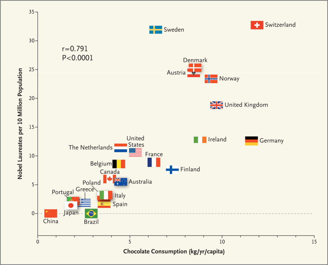
Nobel prizes and chocolate
Simpson’s paradox
etc

2 Machinery

We are interested in representing influence between variables in a non-parametric fashion.

Our main tool to do this will be conditional independence DAGs, and causal use of these. Alternative name: “Bayesian Belief networks”. (Overloads “Bayesian”, so not used here)

2.1 DAGs

DAG: Directed (probabilistic) graphical model. Graph defined, as usual, by a set of vertexes and edges.

$G = (V, E)$

We show the directions of edges by writing them as arrows.

For nodes $X, Y \in V$ we write $X \to Y$ to mean there is a directed edge joining them.

Familiar from, e.g., Structural equation models, hierarchical models, expert systems. General graph theory…

A graph with directed edges, and no cycles. (you cannot return to the same starting node traveling only forward along the arrows)

We need some terminology.

Parents: The parents of a node $X$ in a graph are all nodes joined to it by an incoming arrow, $parents (X) = {Y \in V : Y \to X} .$
Children: similarly, $\operatorname{children}(X)=\{Y\in V:X\rightarrow Y}.$
Co-parent: $\operatorname{coparents}(X)=\{Y\in V:\exists Z\in V \text{ s.t. } X\rightarrow Z\text{ and }Y\rightarrow Z}.$

Ancestors and descendants should be clear as well. For convenience, we define $X \in parents (X)$

2.2 Random variables

I will deal with finite collections of random variables $V$ .

For simplicity of exposition, each of the RVs will be supported on $X_{i} \subset Z$ , so that we may work with pmfs, and write $p (X_{i} | X_{j})$ for the pmf. I may write $p (x_{i} | x_{j})$ to mean $p (X_{i} = x_{i} | X_{j} = x_{j})$ .

Also, we are working with sets of random variables rather than sets of events and the discrete state space reduces the need to discuss sets of events.

Extension to continuous RVs, or arbitrary RVs is trivial for everything I discuss here. (A challenge is if the probabilities are not all strictly positive.)

Motivation in terms of structural models.

$\begin{aligned} X_{6} & = f_{6} (X_{4}, X_{3}, ε_{6}) \\ X_{5} & = f_{5} (X_{4}, X_{3}, ε_{5}) \\ X_{4} & = f_{4} (X_{3}, X_{2}, X_{1}, ε_{4}) \\ X_{3} & = f_{3} (ε_{3}) \\ X_{2} & = f_{2} (X_{1}, ε_{2}) \\ X_{1} & = f_{1} (ε_{1}) \end{aligned}$

Without further information about the forms of $f_{i}$ or $ε_{i}$ , our assumptions have constrained our conditional independence relations to permit a particular factorisation of the mass function:

$p (x_{6}, x_{5}, x_{4}, x_{3}, x_{2}, x_{1}) = p (x_{1}) p (x_{2} | x_{1}) p (x_{3}) p (x_{4} | x_{1}, x_{2}, x_{3}) p (x_{5} | x_{3}, x_{4}) p (x_{6} | x_{3}, x_{4})$

We are “nonparametric” in the sense that working with this conditional factorisation does not require any further parametric assumptions on the model.

However, we would like to proceed from this factorisation to conditional independence, which is non-trivial. Specifically, we would like to know which variables are conditionally independent of others, given such an (assumed) factorisation.

More notation: We write

$X ⊥ Y | Z$

for $X$ independent of $Y$ given $Z$ .

We also use this notation for sets of random variables, and will bold them when it is necessary to emphasise this.

$X ⊥ Y | Z$

Questions:

$X_{2} ⊥ X_{3}$ ?
$X_{2} ⊥ X_{3} | X_{1}$ ?
$X_{2} ⊥ X_{3} | X_{4}$ ?

However, this product notation is not illuminating; we use a graph formalism. That’s where the DAGs come in.

This will proceed in 3 steps

The graphs will describe conditional factorisation relations.
We do some work to construct from these relations some conditional independence relations, which may be read off the graph.
From these relations plus a causal interpretation we derive rules for identification of causal relations
If we get further than that, it will be all about coffee

Anyway, a joint distribution $p (X)$ decomposes according to a directed graph $G$ if we may factor it

$p (X_{1}, X_{2}, \dots, X_{v}) = \prod_{X = 1}^{v} p (X_{i} | parents (X_{i}))$

Uniqueness?

It would be tempting to suppose that a node is independent of its children given its parents or somesuch. But things are not quite so simple.

Questions:

$Sprinkler ⊥ Rain$ ?
$Sprinkler ⊥ Rain | Wet season$ ?
$Sprinkler ⊥ Rain | Wet pavement$ ?
$Sprinkler ⊥ Rain | Wet season, Wet pavement$ ?

To make precise statements about conditional independence relations we do more work.

We need new graph vocabulary and conditional independence vocabulary.

Axiomatic characterisation of conditional independence. (Pearl 2008; Steffen L. Lauritzen 1996).

Theorem: ((Pearl 2008)) For disjoint subsets $W, X, Y, Z \subseteq V .$

Then the relation $\cdot ⊥ \cdot | \cdot$ satisfies the following relations:

$\begin{aligned} X ⊥ Z | Y & \Leftrightarrow & Z ⊥ X | Y & Symmetry \\ X ⊥ Y \cup W | Z & \Rightarrow & X ⊥ Y and X ⊥ W & Decomposition \\ X ⊥ Y \cup W | Z & \Rightarrow & X ⊥ Y | Z \cup W & Weak Union \\ X ⊥ Y | Z and X ⊥ W | Z \cup Y | Z & \Rightarrow & X ⊥ Y \cup W | Z & Contraction \\ X ⊥ Y | Z \cup W and X ⊥ W | Z \cup Y & \Rightarrow & X ⊥ W \cup Y | Z & Intersection & (*) \end{aligned}$

(*) The Intersection axiom only holds for strictly positive distributions.

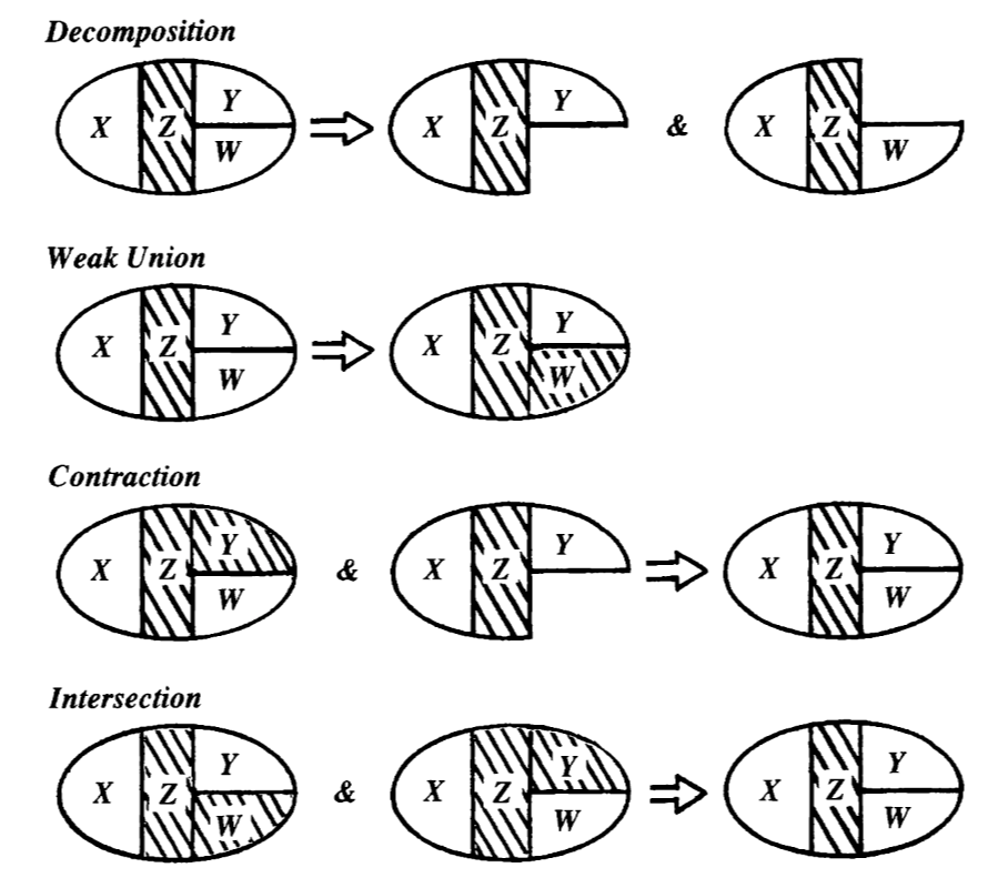
Figure 1: visual intuition of graph axioms, (Pearl 2008)

How can we relate this to the topology of the graph?

The flow of conditional information does not correspond exactly to the marginal factorisation, but it relates. (mention UG connections?)

Definition: A set $S$ blocks a path $π$ from X to Y in a DAG $G$ if either

There is a node $a \in π$ which is not a collider on $π$ such that $a \in S$
There is a node $b \in π$ which is a collider on $π$ and $descendants (b) \cap S = \emptyset$

If a path is not blocked, it is active.

Definition: A set $S$ d-separates two subsets of nodes $X, Y \subseteq G$ if it blocks every path between any pair of nodes $(A, B)$ such that $A \in X, B \in Y .$

This looks ghastly and unintuitive, but we have to live with it because it is the shortest path to making simple statements about conditional independence DAGs without horrible circumlocutions, or starting from undirected graphs, which is tedious.

Theorem: (Pearl 2008; Steffen L. Lauritzen 1996). If the joint distribution of $V$ factorises according to the DAG $G$ then for two subsets of variables $X ⊥ Y | S$ iff $S$ d-separates $X$ and $Y$ .

This puts us in a position to make non-awful, more intuitive statements about the conditional independence relationships that we may read off the DAG.

Corollary: The DAG Markov property.

$X ⊥ descendants (X)^{C} | parents (X)$

Corollary: The DAG Markov blanket.

Define

$blanket (X) := parents (X) \cup children (X) \cup coparents (X)$

Then

$X ⊥ blanket (X)^{C} | blanket (X)$

3 Causal interpretation

Finally!

We have a DAG $G$ and a set of variables $V$ to which we wish to give a causal interpretation.

Assume

The $V$ factors according to $G$
$X \to Y$ means “causes” (The Causal Markov property)
We additionally assume faithfulness, that is, that $X ↭ Y$ iff there is a path connecting them.

So, are we done? Only if correlation equals causation.

Figure 5: Chocolate and Nobel prizes, Messerli (2012)

We add the additional condition that

all the relevant variables are included in the graph. (We coyly avoid making this precise)

The BBC raised one possible confounding variable:

[…] Eric Cornell, who won the Nobel Prize in Physics in 2001, told Reuters “I attribute essentially all my success to the very large amount of chocolate that I consume. Personally I feel that milk chocolate makes you stupid… dark chocolate is the way to go. It’s one thing if you want a medicine or chemistry Nobel Prize but if you want a physics Nobel Prize it pretty much has got to be dark chocolate.”

Finally, we need to discuss the relationship between conditional dependence and causal effect. This is the difference between, say,

$P (Wet pavement | Sprinkler = o n)$

and

$P (Wet pavement | do (Sprinkler = o n))$

Called “truncated factorization” in the paper. $do$ -calculus and graph surgery.

If we know $P$ , this is relatively easy. Marginalize out all influences on the causal variable of interest, which we show graphically as wiping out a link.

Now suppose we are not given complete knowledge of $P$ , but only some of the conditional distributions. (There are unobservable variables). This is the setup of observational studies and epidemiology and so on.

What variables must we know the conditional distributions of in order to know the conditional effect? That is, we call a set of covariates $S$ an admissible set (or sufficient set) with respect to identifying the effect of $X$ on $Y$ if

$p (Y = y | d o (X = x)) = \sum_{s} P (Y = y | X = x, S = s) P (S = s)$

Criterion 1: The parents of a cause are an admissible set (Pearl 2009a).

Criterion 2: The back door criterion.

A set $S$ such that

$S \cap descendants (X) = \emptyset$
$S$ blocks all paths which start with an arrow into $X$

This is a sufficient condition.

Causal properties of sufficient sets:

$P (Y = y | do (X = x), S = s) = P (Y = y | X = x, S = s)$

Hence

$P (Y = y | do (X = x), S = s) = \sum_{s} P (Y = y | X = x, S = s) P (S = s)$

4 Examples

Figure 6: Social influence model in Shalizi and Thomas (2011)

$i, j$ are individuals,
$Z$ denote observed traits,
$X$ denote latent traits
$Y$ denote observed outcomes
$A$ is a network tie

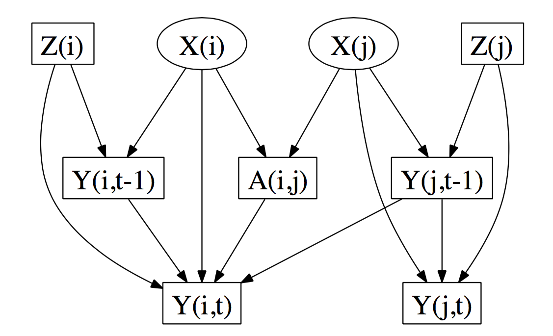
$X_{i}$ d-separates $Y_{i} (t)$ from $A_{i j}$ . Since $X_{i}$ is latent and unobserved, $Y_{i} (t) \leftarrow X_{i} \to A_{i j}$ is a confounding path from $Y_{i} (t)$ to $A_{i j}$ . Likewise $Y_{j} (t - 1) \leftarrow X_{j} \to A_{i j}$ is a confounding path from $Y_{i} (t - 1)$ to $A_{i j}$ . Thus, $Y_{i} (t)$ and $Y_{i} (t - 1)$ are d-connected when conditioning on all the observed (boxed) variables […] . Hence the direct effect of $Y_{i} (t)$ on $Y_{i} (t - 1)$ is not identifiable

5 Recommended reading

People recommend Koller and Friedman, which includes many different flavours of DAG model and many different methods, (Koller and Friedman 2009) but it didn’t suit me, being somehow too detailed and too non-specific at the same time.

Spirtes et al (Spirtes, Glymour, and Scheines 2001) and Pearl (Pearl 2009a) are readable. See also Pearl’s edited highlights (Pearl 2009b). Lauritzen ((Steffen L. Lauritzen 1996)) is clear but the details of the constructions are long and detailed and more general than here. (Partially directed graphs.)

Lauritzen’s shorter introduction (Steffen L. Lauritzen 2000) is nice if you can get it; Not overwhelming, starts with a slightly more general formalism (DAGs as a special case of PDAGs, moral graphs everywhere). Murphy’s textbook (Murphy 2012) has a minimal introduction intermingled with some related models, with a more ML, “expert systems”-flavoured and more Bayesian formalism.

6 References

Aral, Muchnik, and Sundararajan. 2009. “Distinguishing Influence-Based Contagion from Homophily-Driven Diffusion in Dynamic Networks.” Proceedings of the National Academy of Sciences.

Arnold, Castillo, and Sarabia. 1999. Conditional Specification of Statistical Models.

Bareinboim, and Pearl. 2016. “Causal Inference and the Data-Fusion Problem.” Proceedings of the National Academy of Sciences.

Bareinboim, Tian, and Pearl. 2014. “Recovering from Selection Bias in Causal and Statistical Inference.” In AAAI.

Bloniarz, Liu, Zhang, et al. 2015. “Lasso Adjustments of Treatment Effect Estimates in Randomized Experiments.” arXiv:1507.03652 [Math, Stat].

Brodersen, Gallusser, Koehler, et al. 2015. “Inferring Causal Impact Using Bayesian Structural Time-Series Models.” The Annals of Applied Statistics.

Bühlmann. 2013. “Causal Statistical Inference in High Dimensions.” Mathematical Methods of Operations Research.

Bühlmann, Kalisch, and Meier. 2014. “High-Dimensional Statistics with a View Toward Applications in Biology.” Annual Review of Statistics and Its Application.

Bühlmann, Peters, Ernest, et al. 2014. “Predicting Causal Effects in High-Dimensional Settings.”

Bühlmann, Rütimann, and Kalisch. 2013. “Controlling False Positive Selections in High-Dimensional Regression and Causal Inference.” Statistical Methods in Medical Research.

Chen, and Pearl. 2012. “Regression and Causation: A Critical Examination of Econometric Textbooks.”

Claassen, Mooij, and Heskes. 2014. “Proof Supplement - Learning Sparse Causal Models Is Not NP-Hard (UAI2013).” arXiv:1411.1557 [Stat].

Colombo, Maathuis, Kalisch, et al. 2012. “Learning High-Dimensional Directed Acyclic Graphs with Latent and Selection Variables.” The Annals of Statistics.

De Luna, Waernbaum, and Richardson. 2011. “Covariate Selection for the Nonparametric Estimation of an Average Treatment Effect.” Biometrika.

Elwert. 2013. “Graphical Causal Models.” In Handbook of Causal Analysis for Social Research. Handbooks of Sociology and Social Research.

Ernest, and Bühlmann. 2014. “Marginal Integration for Fully Robust Causal Inference.” arXiv:1405.1868 [Stat].

Gelman. 2010. “Causality and Statistical Learning.” American Journal of Sociology.

Hinton, Osindero, and Bao. 2005. “Learning Causally Linked Markov Random Fields.” In Proceedings of the 10th International Workshop on Artificial Intelligence and Statistics.

Jordan, Michael Irwin. 1999. Learning in Graphical Models.

Jordan, Michael I., and Weiss. 2002a. “Graphical Models: Probabilistic Inference.” The Handbook of Brain Theory and Neural Networks.

———. 2002b. “Probabilistic Inference in Graphical Models.” Handbook of Neural Networks and Brain Theory.

Kalisch, and Bühlmann. 2007. “Estimating High-Dimensional Directed Acyclic Graphs with the PC-Algorithm.” Journal of Machine Learning Research.

Kennedy. 2015. “Semiparametric Theory and Empirical Processes in Causal Inference.” arXiv Preprint arXiv:1510.04740.

Kim, and Pearl. 1983. “A Computational Model for Causal and Diagnostic Reasoning in Inference Systems.” In IJCAI.

Koller, and Friedman. 2009. Probabilistic Graphical Models : Principles and Techniques.

Lauritzen, Steffen L. 1996. Graphical Models. Oxford Statistical Science Series.

———. 2000. “Causal Inference from Graphical Models.” In Complex Stochastic Systems.

Lauritzen, S. L., and Spiegelhalter. 1988. “Local Computations with Probabilities on Graphical Structures and Their Application to Expert Systems.” Journal of the Royal Statistical Society. Series B (Methodological).

Maathuis, and Colombo. 2013. “A Generalized Backdoor Criterion.” arXiv Preprint arXiv:1307.5636.

Maathuis, Colombo, Kalisch, et al. 2010. “Predicting Causal Effects in Large-Scale Systems from Observational Data.” Nature Methods.

Maathuis, Kalisch, and Bühlmann. 2009. “Estimating High-Dimensional Intervention Effects from Observational Data.” The Annals of Statistics.

Marbach, Prill, Schaffter, et al. 2010. “Revealing Strengths and Weaknesses of Methods for Gene Network Inference.” Proceedings of the National Academy of Sciences.

Messerli. 2012. “Chocolate Consumption, Cognitive Function, and Nobel Laureates.” New England Journal of Medicine.

Mihalkova, and Mooney. 2007. “Bottom-up Learning of Markov Logic Network Structure.” In Proceedings of the 24th International Conference on Machine Learning.

Montanari. 2011. “Lecture Notes for Stat 375 Inference in Graphical Models.”

Murphy. 2012. Machine learning: a probabilistic perspective. Adaptive computation and machine learning series.

Neapolitan. 2003. Learning Bayesian Networks.

Noel, and Nyhan. 2011. “The ‘Unfriending’ Problem: The Consequences of Homophily in Friendship Retention for Causal Estimates of Social Influence.” Social Networks.

Pearl. 1982. “Reverend Bayes on Inference Engines: A Distributed Hierarchical Approach.” In Proceedings of the Second AAAI Conference on Artificial Intelligence. AAAI’82.

———. 1986. “Fusion, Propagation, and Structuring in Belief Networks.” Artificial Intelligence.

———. 2008. Probabilistic reasoning in intelligent systems: networks of plausible inference. The Morgan Kaufmann series in representation and reasoning.

———. 2009a. “Causal Inference in Statistics: An Overview.” Statistics Surveys.

———. 2009b. Causality: Models, Reasoning and Inference.

Peters, Bühlmann, and Meinshausen. 2015. “Causal Inference Using Invariant Prediction: Identification and Confidence Intervals.” arXiv:1501.01332 [Stat].

Raginsky. 2011. “Directed Information and Pearl’s Causal Calculus.” In 2011 49th Annual Allerton Conference on Communication, Control, and Computing (Allerton).

Rubin, and Waterman. 2006. “Estimating the Causal Effects of Marketing Interventions Using Propensity Score Methodology.” Statistical Science.

Sauer, and VanderWeele. 2013. Use of Directed Acyclic Graphs.

Shalizi, and McFowland III. 2016. “Controlling for Latent Homophily in Social Networks Through Inferring Latent Locations.” arXiv:1607.06565 [Physics, Stat].

Shalizi, and Thomas. 2011. “Homophily and Contagion Are Generically Confounded in Observational Social Network Studies.” Sociological Methods & Research.

Shpitser, and Pearl. 2008. “Complete Identification Methods for the Causal Hierarchy.” The Journal of Machine Learning Research.

Shpitser, and Tchetgen. 2014. “Causal Inference with a Graphical Hierarchy of Interventions.” arXiv:1411.2127 [Stat].

Smith, and Eisner. 2008. “Dependency Parsing by Belief Propagation.” In Proceedings of the Conference on Empirical Methods in Natural Language Processing.

Spirtes, Glymour, and Scheines. 2001. Causation, Prediction, and Search. Adaptive Computation and Machine Learning.

Vansteelandt, Bekaert, and Claeskens. 2012. “On Model Selection and Model Misspecification in Causal Inference.” Statistical Methods in Medical Research.

Wright. 1934. “The Method of Path Coefficients.” The Annals of Mathematical Statistics.

Yedidia, Freeman, and Weiss. 2003. “Understanding Belief Propagation and Its Generalizations.” In Exploring Artificial Intelligence in the New Millennium.

Zhang, Peters, Janzing, et al. 2012. “Kernel-Based Conditional Independence Test and Application in Causal Discovery.” arXiv:1202.3775 [Cs, Stat].