Bayesian nonparametric statistics
Updating more dimensions than datapoints
2016-05-30 — 2025-08-14
Wherein Infinite-Dimensional Parameter Spaces Are Invoked and Posterior Updates Are Expressed via Radon–Nikodym Derivatives, Gaussian Processes and Dirichlet Measure Priors Are Employed, and Consistency Pitfalls for Functional Models Are Noted.

“Nonparametric” Bayes refers to Bayesian inference in which the parameters are infinite-dimensional (I don’t like that term). There’s a connection to predictive Bayes that I’d like to understand better.
1 Useful stochastic processes
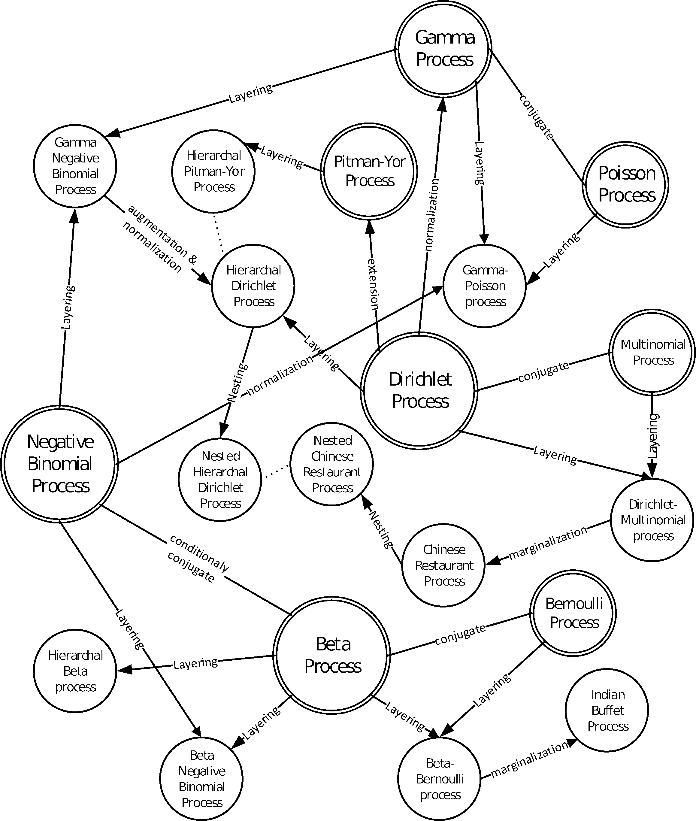
Dirichlet priors and other measure priors, Gaussian process regression, reparameterizations etc. 🚧TODO🚧
2 Posterior updates in infinite dimensions
For now, this is just a bookmark to the general measure-theoretic notation that, in principle, unifies the various Bayesian nonparametric methods. A textbook on the general theory is Schervish (2012). Chapter 1 of Matthews (2017) gives a compact introduction.
Particular applications are outlined in Matthews (2017) (see Gaussian process regression) and Stuart (2010) (see inverse problems).
A brief introduction to the measure-theoretic notation we need in infinite-dimensional Hilbert space settings is in Alexanderian (2021), which gives Bayes’ formula as \[ \frac{d \mu_{\text {post }}^{y}}{d \mu_{\text {pr }}} \propto \pi_{\text {like }}(\boldsymbol{y} \mid m), \] where the left-hand side is the Radon–Nikodym derivative of \(\mu_{\text {post }}^{y}\) with respect to \(\mu_{\text {pr }}\).
They observe
Note that in the finite-dimensional setting the abstract form of the Bayes’ formula above can be reduced to the familiar form of Bayes’ formula in terms of PDFs. Specifically, working in finite dimensions, with \(\mu_{\mathrm{pr}}\) and \(\mu_{\mathrm{post}}^{y}\) that are absolutely continuous with respect to the Lebesgue measure \(\lambda\), the prior and posterior measures admit Lebesgue densities \(\pi_{\mathrm{pr}}\) and \(\pi_{\text {post }}\), respectively. Then, we note \[ \pi_{\mathrm{post}}(m \mid \boldsymbol{y})=\frac{d \mu_{\mathrm{post}}^{y}}{d \lambda}(m)=\frac{d \mu_{\mathrm{post}}^{y}}{d \mu_{\mathrm{pr}}}(m) \frac{d \mu_{\mathrm{pr}}}{d \lambda}(m) \propto \pi_{\mathrm{like}}(\boldsymbol{y} \mid m) \pi_{\mathrm{pr}}(m) \]
3 Bayesian consistency
Consistency turns out to be tricky for functional models. I’m not an expert on consistency, but see Cox (1993) for some warnings about what can go wrong, and Florens and Simoni (2016); Knapik, van der Vaart, and van Zanten (2011) for some remedies. tl;dr: posterior credible intervals arising from over-tight priors may never cover the frequentist estimate. Further reading on this is in some classic refs: (Diaconis and Freedman 1986; Freedman 1999; Kleijn and van der Vaart 2006).