Coincidences and computation

1.1 Reviewer abstract

I know a bit about random neural networks but less about computational complexity. I put all my notes in the “abstract” in the hope that it will be useful for others with my background, and because it might expose my errors of reasoning. If you already know about such things, you can skip to the end.

Note: Since there was some notation clash between the original blog post and this paper, I introduce compromise notation. Dunbar’s \(n\) is \(m\).

Neyman and coworkers at the ARC would like to formalise when a neural network has “discovered a way of doing things that we can study” in terms of when an surprising behaviour is susceptible to an easy verification. Their motivation is a computational operationalisation of Tim Gowers’s no coincidence principle

If an apparently outrageous coincidence happens in mathematics, then there is a reason for it.

They see his no-coincidence principle and counter with the computational no-coincidence conjecture (CNCC), which uses computational-complexity machinery in the space of random functions to turn it into something we can imagine operationalizing.

I don’t come from computational complexity, so I’ll spell the computational no-coincidence conjecture out here for myself and others like me. I’ll give it in the form we need for the paper — abstract enough to cover the cases we care about but concrete enough to be pedagogical. Suppose we have a universe of functions (circuits, neural networks, Turing machines), and suppose that this universe comes equipped with a probability measure so we can draw functions at random from this universe of functions.

Working with random functions has some annoying technicalities; let’s barrel through them briskly. Because I’m an ML guy, I’ll assume we only care about real vector functions — that’s specific enough for me to keep in my head, and it’s worked for me so far. Call this universe \(\Omega\). Each function \(f \in \Omega\) is a map from¹ \(\mathbb{R}^{m}\to\mathbb{R}^{m}\) i.e. we have an \(m\)-dimensional input space and an \(m\)-dimensional output space.². We call the probability measure \(\mu\)³ and for technical probability-theory reasons we want a \(\sigma\)-algebra defined (“\(\mathcal{F}\)”) over our function space so that things don’t go haywire when we attempt to compute probabilities of “things” in this function space. This is generally easy for discrete function spaces but gets tedious for function spaces between vectors over continuous fields like the reals. \(\mathcal{F}\) needs to hold all the sets over which we might attempt to compute probabilities. We wrap these up in a probability tuple \((\Omega, \mu, \mathcal{F})\) that lets us do probability stuff in a well-posed way to our universe of functions.

There are various desirable properties for this function space.

1. For our phenomena of interest, we should be able to guesstimate how likely it is to be observed by chance, i.e. we should be able to bound probabilities of rare events of interest (we will come back to this)
2. We should be required to spend the absolute minimum of time arsing about with \(\sigma\)-algebras and other distracting technical machinery.
3. The function space should map cleanly onto some class of functions we care about (e.g. it should be “easy” to interpret things from our function space as neural nets or Turing machines or what-have-you)

The original blog post addressed these desiderata by dealing with the space of random reversible circuits, i.e. random Boolean functions with some nice structure from \(\{0,1\}^{3n}\to \{0,1\}^{3n}\) (i.e. \(m=3n\)). These objects are discrete, so desideratum (2) is easy. They have a neat approximation in terms of random permutations, so that’s (1) dealt with. (3) is addressed by deciding we care about Boolean circuits for now, and computer scientists are comfortable thinking about the space of Boolean circuits as a toy model for all kinds of things like formal logic and… other discrete problems that computer scientists care about.

Let’s fix on the setting of that Neyman blog post: random deep reversible Boolean circuits \(f: \{0,1\}^{3n} \to \{0,1\}^{3n}\). The distribution is concrete — e.g., pick a random sequence of 3-bit reversible gates, arranged in layers that touch all wires, to a given depth. For large enough depth, such circuits behave pseudorandomly: recent results apparently show they achieve strong \(k\)-wise independence.

This motivates modelling a deep random reversible circuit as though it were drawn uniformly from the symmetric group on \(\{0,1\}^{3n}\), \(\mathrm{Sym}(\{0,1\}^{3n})\).⁴ So that solves (1) for us. There are a lot of permutations, but we’ve studied the crap out of them, so that should be manageable. We have a simple, albeit approximate, distribution for circuits here.

To bring us back to the main goal: we’re doing this because we want a good notion of the distributions of such functions — circuits that might, if we squint, look a bit like deductions about the world — so we can quantify what it means for their behaviour to be remarkable and what it might mean to explain remarkable behaviour \(P\). We are working toward the idea that something is remarkable if its behaviour is “outrageously coincidental”, which we can now gloss as very low probability under the null distribution.

We focus on properties \(P\) that talk about the mapping from inputs to outputs across the entire admissible input set. Formally:

\(P(f)\) means : there is no input \(x\) such that \(p_{\text{in}}(x)\) and \(p_{\text{out}}(f(x))\) are both true.

Here \(p_{\text{in}} : \{0,1\}^\ell \to \{\text{True},\text{False}\}\) and \(p_{\text{out}} : \{0,1\}^m \to \{\text{True},\text{False}\}\) are Boolean predicates on inputs and outputs, respectively.⁵ In Neyman’s example, let’s label it \(P^{(0)}\). \(p^0_{\text{in}}(x)\) is “the last \(n\) bits of \(x\) are all 0”, and \(p^0_{\text{out}}(y)\) is the same condition on \(y\). The \(P^{(0)}\) in Neyman’s blog post says: for every input whose last \(n\) bits are 0, the corresponding output’s last \(n\) bits are not all 0.

Spelling it out for myself: if there’s even one input in the \(p^0_{\text{in}}\) set whose output also lies in \(p^0_{\text{out}}\), then \(P^{(0)}(f)\) fails. That’s why a property like “output bit \(i > 2n\) is always 1 for all \(p_{\text{in}}\) inputs” is enough to guarantee \(P^{(0)}(f)\) — it eliminates the possibility of the output’s last \(n\) bits all being zero.

There are \(2^{3n}\) binary strings of length \(3n\). How many end in \(n\) zeros? \(2^{2n}\) of those. Permutations \(f\) that never produce a string ending in \(n\) zeros from a string ending in \(n\) zeros? Feels… enumerable. If we model it as something like a random process, it feels like we can estimate the probability of that event, and in fact the probability that a randomly chosen permutation does that, \[ (1-2^{-n})^{2^{2n}} \approx e^{-2^n} \] In reality, the reversible-circuit distribution isn’t exactly uniform over all permutations — structured outliers exist — but for the purposes of bounding the probability of \(P^{(0)}(f)\) they’re probably negligible, so this simple form will do for the moment. So if a randomly chosen circuit has this property, I’d be astonished if \(n\) were bigger than the number of fingers I have.

We’re nearly at the computational no-coincidence conjecture — hang on; we want to use this machinery to capture “structure” in functions that explains outrageous coincidences. We’ll say an outrageous coincidence for a function \(f\) is explained by structure if there exists an advice string, \(\pi(f)\), and a verification algorithm \(V(f, \pi(f))\) that can quickly check \(P(f)\). “Quickly” means polynomial time in the “size” of \(f\), which can be some count of the number of gates.

The computational no-coincidence conjecture is that

1. For all \(f\) such that \(P(f)\) is true, \(V(f, \pi(f))=\textrm{true}\) [TODO clarify]
2. For 99% of \(f\) such that \(P(f)\) is false, there is no \(\pi(f)\) that makes \(V(f,\pi(f))=\textrm{true}\). [TODO clarify]

The 99% clause prevents us from breaking the computational complexity hierarchy. We can’t allow perfect classifiers here.

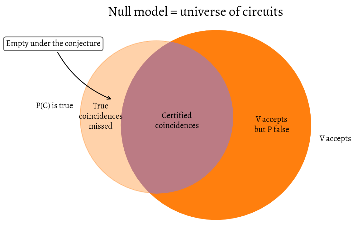
Meanwhile, (a) does the work of “explaining” structure. It says that if we can always find an advice (let’s gloss that as a compact demonstration that the structure is real) for a fixed, outrageously unlikely property \(P\) (and for a fixed \(\Omega\), etc.), then the verifier \(V\), given that advice, has perfect recall (and good specificity) over the set of all random functions. In set diagrams, we claim that the set of functions \(f\) that satisfy \(P(f)\) but for which no proof \(\pi(f)\) will persuade our verifier is empty.

So! A formalization of the conjecture that all coincidences must be explainable.

import matplotlib.pyplot as plt
import matplotlib as mpl
from matplotlib_set_diagrams import EulerDiagram
from livingthing.matplotlib_style import set_livingthing_style, reset_default_style

set_livingthing_style()

P_true_size = 0.13
V_accepts_size = 0.20
intersection_size = 0.09

subset_sizes = {
    (1, 0): P_true_size - intersection_size,   # A only: "10"
    (0, 1): V_accepts_size - intersection_size,# B only: "01"
    (1, 1): intersection_size,                 # A∩B:   "11"
}

subset_labels = {
    (1, 0): "True\ncoincidences\nmissed",
    (0, 1): "V accepts\nbut P false",
    (1, 1): "Certified\ncoincidences",
}

fig, ax = plt.subplots(figsize=(6, 5))

# Try a cost objective that preserves *relative* sizes nicely.
diagram = EulerDiagram(
    subset_sizes,
    subset_labels=subset_labels,
    set_labels=["P(C) is true", "V accepts"],
    cost_function_objective="relative",   # good for preserving ordering
    verbose=False,
    ax=ax,
)
for key, text_artist in diagram.subset_label_artists.items():
    text_artist.set_color("black")

# Highlight the 10 region directly
artist_10 = diagram.subset_artists[(True, False)]
artist_10.set_facecolor("tab:orange")
artist_10.set_alpha(0.35)
artist_10.set_edgecolor("tab:orange")

# Use shapely centroid for a precise callout
geom_10 = diagram.subset_geometries[(True, False)]
x, y = geom_10.centroid.x, geom_10.centroid.y
ax.annotate(
    "Empty under the conjecture",
    xy=(x, y+0.03),
    xycoords="data",
    xytext=(-15, 65),
    textcoords="offset points",
    ha="right",
    bbox=dict(
      boxstyle="round,pad=0.3", fc="w", ec="0.4"),
    arrowprops=dict(
      arrowstyle="->",
      connectionstyle="arc3,rad=0.2"),
)

ax.set_title("Null model = universe of circuits")
ax.set_axis_off()
plt.tight_layout()
plt.show()
# print(f"savefig.transparent {mpl.rcParams['savefig.transparent']}")
# print(f"figure.facecolor {mpl.rcParams['figure.facecolor']}")
# print(f"axes.facecolor {mpl.rcParams['axes.facecolor"]}")
# print(f"fig patch {fig.get_facecolor(), fig.get_alpha()}")
# print(f"ax patch {ax.get_facecolor(), ax.get_alpha()}")
# print(f"fig facecolor {fig.get_facecolor()}")   # expect rgba with alpha 0
# print(f"ax facecolor {ax.get_facecolor()}")    # expect alpha 0

# (Optional sanity check)
# print("Radii:", diagram.radii)  # different radii reflect set totals A vs B

We can now see what a “structural” explanation of \(P^{(0)}(f)\) might look like. For instance, suppose there exists an output bit in position \(i > 2n\) — i.e., one of the final \(n\) bits — such that for every input whose last \(n\) bits are all zero, the circuit flips that bit from 0 to 1 on the first layer and never changes it again. This ensures that any input in the \(p^0_{\text{in}}\) set (last \(n\) bits zero) will produce an output where bit \(i\) is fixed to 1, so the output’s last \(n\) bits can never all be zero. In other words, \(P(f)\) holds for a simple, structural reason.

In the CNCP world, this is a kind of case where the “advice” \(\pi(f)\) could be very compact — e.g., “bit \(i\) is constant-1 across the entire \(p^0_{\text{in}}\) domain” — and the verifier \(V\) could check it in polynomial time by evaluating the circuit on just the relevant subset of inputs. The conjecture’s claim, I understand, is that all circuits satisfying \(P\) have some succinct, checkable \(\pi\), not just this toy case.

1.2 Review

This paper does a lot of hard work to find criteria and conditions under which wide, deep neural networks give us a tractable null distribution for producing Computational No-Coincidence Conjecture results. It supplies one such example plus many useful auxiliary results that would help us produce more. As far as I understand the conjecture, this paper mostly adapts it to neural-network domains, which seems useful for making progress. It is, IMO, clearly written, with some rough edges that I suspect come from the paper sitting at the edge of two fields with strong opinions about terminology; we may not all agree on how rough those edges are.

I have examined the technical results at a surface level, and they seem credible, but errors could have escaped me.

I have questions.