Ergodicity economics

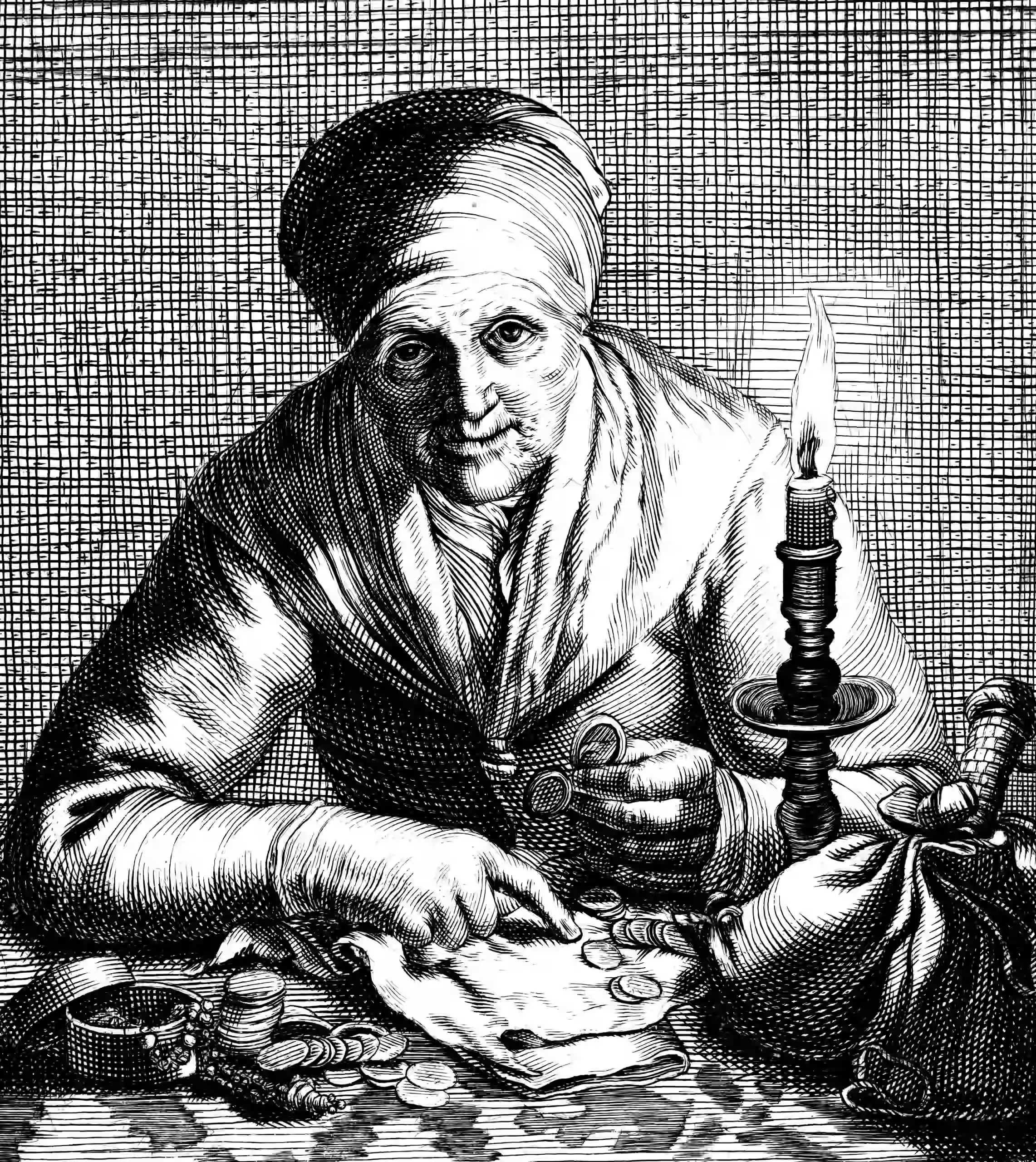
An optionality-flavoured variant of economic decision theory (Peters 2019).

A system is ergodic if averaging an observable across many parallel trajectories at a single moment gives the same answer as averaging it along one trajectory over time — i.e., “many people now” and “one person across many years” agree.

Many systems we care about are non-ergodic. Peters’ canonical counter-example is a repeated coin flip bet: each round, my wealth \(W\) is multiplied by \(1.5\) if the coin lands heads and by \(0.6\) if it lands tails. The coin is fair; whether the gamble is fair depends on which average we care about.¹

The ensemble average surveys many of us playing in parallel, at a fixed round \(n\). The mean multiplier per round is the arithmetic average of the two outcomes, so

\[\mathbb{E}[W_n] \;=\; W_0 \left(\frac{1.5 + 0.6}{2}\right)^{\!n} \;=\; W_0 \times 1.05^n .\]

On average, the gamble is better than fair: a 5% edge per round, compounding! That sounds like a free lunch.

The time average follows one of us (e.g., me) playing many rounds in sequence. The law of large numbers grants me heads on about half the rounds and tails on the other half, so

\[W_n \;\approx\; W_0 \,(1.5 \times 0.6)^{n/2} \;=\; W_0 \times 0.9^{n/2} \;\approx\; W_0 \times 0.95^n .\]

On this average, the same gamble is worse than fair: my wealth decays by about 5% per round until I have nothing.

Both calculations are correct; they disagree because repeated multiplication can be understood in terms of the geometric mean of the multipliers, \(\sqrt{1.5 \times 0.6} \approx 0.95\), which is less than the arithmetic mean \(1.05\). That disagreement is all that non-ergodicity means here. After 100 rounds the ensemble mean is \(1.05^{100}\,W_0 \approx 130\,W_0\), while the median player holds \(0.9^{50}\,W_0\), about half a percent of their starting stake. The mean is propped up by an exponentially rare minority of heads-heavy histories. This is not reassuring to me as a player since I get to live only one history, and that is very unlikely to be the lucky one.

cf Garrabrant’s Geometric Rationality.

Peters argues that under non-ergodicity, expected utility optimizes the wrong average. In our coin flip with \(\mathbb{E}[\log r] < 0\) almost every trajectory decays exponentially, so the time average of wealth is \(0\), and in a gamble with \(\mathbb{E}[\log r] > 0\) it would be \(\infty\) instead. This is degenerate either way — useless for ranking one gamble against another. The observable with a finite, informative limit is the growth rate, \(\tfrac{1}{n}\log(W_n/W_0) \to \mathbb{E}[\log r] \approx \log 0.95\) per round. Almost every trajectory shares this growth rate. The growth rate, unlike wealth, is ergodic: its time average agrees with its expectation, so its expectation describes what happens to a single player, which is the property that prompted us to take expectations in the first place. Ergodicity economics says to optimize that number: expected wealth endorses the coin flip above, time-average growth refuses it. Under multiplicative dynamics, the growth rate is an expected log, so this happens to coincide with log utility. Neatly, the log emerges naturally from the dynamics, rather than being given, so that is nice, I suppose.

Contrast an additive variant of the gamble, with stakes that do not scale with our wealth: heads wins us fifty dollars, tails loses us forty, whatever our balance. The gain per round is then the ergodic observable — \((W_n - W_0)/n \to \tfrac12(50) - \tfrac12(40) = 5\) dollars along almost every (solvent) trajectory, which is also its expectation — so ranking gambles by time-average growth is the same as ranking them by expected wealth. Maximizing time-average growth over how much we stake is the Kelly criterion, which disfavours any action that risks ejecting the agent from the support of viable trajectories.