X is Yer than Z

March 2, 2021 — June 22, 2020

how do science

statistics

Notes on a simple and essential part of how we talk about the world that we frequently do not think through even though it is, rhetorically speaking, a gigantic chunk of what we do in business and politics. It is not complex, but surprisingly hard to get an intuitive grip on. This is the basic-but-easy-to-confuse question, “what we mean when we say that X is Yer than Z, when X and Y are both groups?”

If I claim that this apple is has a larger diameter than that orange, what I must mean is simple, and if we want to verify my claim, we can measure the fruit in question if we have a reasonably reliable tape measure and a steady hand. So much not easy to misunderstand.

But imagine not that I am now talking about larger quantities of fruit. Like “the apples in this barrel are bigger than the apples in that barrel. “The apples of the Pink Lady harvest in Australia in 2018 are bigger than the tangerines of Java in 2017.” “Clementines are smaller than pomellos.”

(Why do I care so much about fruits? Fruits are not my primary object here. This loose talk vexes me most of all when it is in statements about humans, or of risk where the failure modes of doing it wrong are bad. We will get to those.)

See Figure @ref(fig:pie) for example:

Code

#par(mar = c(0, 1, 0, 1))
plot(
  #c(
    function(x) dnorm(x),
  #  function(x) dnorm(x, 1)
  #),
  -2, 2,
)
plot(
  #c(
    function(x) dnorm(x),
  #  function(x) dnorm(x, 1)
  #),
  -2, 2,
)

1 First moment

🍎 🍊

2 Cohen’s \(d\) for normally distributed populations

🏗

3 On bell curves

So far we have looked at Gaussian distributions, a.k.a. “bell curves”. Gaussian distributions are powerful and useful distributions and they pop up all over the place for all manner of reasons. They do have certain implications to be aware of.

Firstly, a common justification for Gaussian distributions is the idea that they arise from huge numbers of interacting underlying non-Gaussian random variables interacting in a certain class of complicated ways. In a sense when we assume a population has a Gaussian distribution over some feature of interest we are arguing that there are some complicated underlying factors that we cannot (or do not care to) disentangle. ¹ The default (although not the only) justification of a Gaussian distribution to model our population is the assumption that inner workings of our phenomenon of interest are some entangled snarl of complicated interacting factors that we can comprehend only when we smash them all together and ignore the details. Gaussian distributions are indeed the ones that are maximally hard to disentangle in a certain sense being maximal entropy distributions (see e.g. Independent Component Analysis, which uses non-Gaussianity to disentangle variabls from one another, or the classical error-in-identifiability results Reiersol (1950).)

Specifically, the bell curve amounts to the assumptions that there are no Gaussian sub-populations. A mixture of Gaussian populations is not Gaussian.

Another justification, a Gaussian distribution for some feature in a population could imply that we are making an expedient approximation; Gaussian distributions are computationally easy, in the sense that statistics are easy to do if you cross your fingers and pretend things are Gaussian. So another implication of a Gaussian distribution is that reality was too complicated so I pretended. This was especially important back when computers were expensive and data was scarce, but is less often so important these days these days. (Although see Gaussian process regression.) For large-data multivariate density estimates, assuming Gaussian distributions in the face of facts can be an expensive mistake. That said, approximation is a completely legitimate thing to do; all statistics and maybe all consciousness is statistical approximation. We merely need to be aware that we are doing it, and check our assumptions to make sure this convenience is justified by the task and constraints at hand. If we do not check those assumptions, we are assuming that our model is not important enough to make accurate. Assuming Gaussian distributions in the face of facts can be an expensive mistake, e.g. global financial-crisis-level mistake. A COVID-19 mistake.

tl;dr Gaussian distributions are important statistical workhorses, but much of modern statistics is a delicate dance toward and away from Gaussian distributions. Declaring things to just be Gaussian is like declaring all food to be soylent.

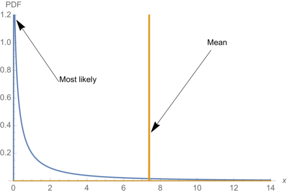
In extreme cases assuming oversimplification such as this can tell you almost nothing about the quantity of interest, e.g. missing a whole pandemic. Most of the “action” in a log-normal distribution, for example, is far from the mean.

Figure 1: A log-normal distribution from Nassim Taleb’s grumpy blog post

But so much is standard statistics first-year statistics.

4 Higher moments

5 Relative distributions

See Reldist (Mark Stephen Handcock and Morris 1999).

6 In the wild

Here are two (AFAICT politically opposed bloggers) who seem to do violence to this concept in a discussion of on race and IQ: Brink Lindsey and Kevin Drum.
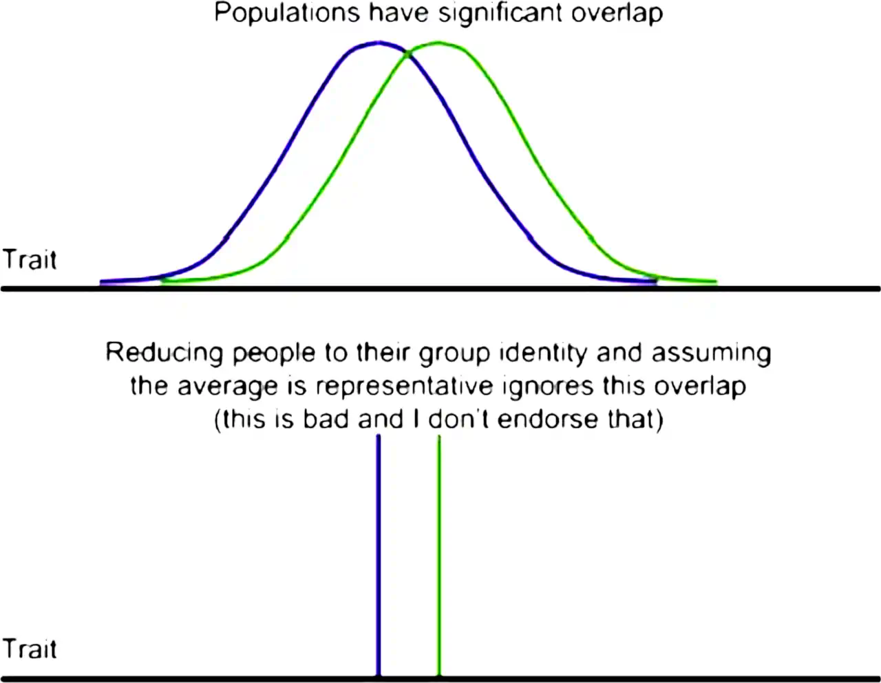
gender is another fraught area. Many examples available. The notorious James Damore Memo (“Inside the ideological echo chamber”) is one of them. It has flaws IMO, but it also has an unusual virtue, which is making a common confusion explicit via the following diagram, wherein it distinguishes reasoning based on the mean (or some other characterisation of a distribution) from reasoning based on the whole distributions:

Figure 2

I suspect that essay of falling prey some different logical fallacies instead, but that is a suspicion that another version of myself would have to verify, i.e. who has time to commit to understanding the office dynamics of Californian dotcoms.
Eliezer Yudkowsky’s essay, How an algorithm feels from the inside is an argument about why our human brains may find categorisation hard.

7 TODO

Mention that the surprising simplicty of comparison of Bernoulli RVs
All of which is not to say that X is never Yer than Z. c.f. The Whole City Is Center, Nootropics Survey 2020 Results
Tails of Great Soccer Players

Now think about interaction effects.

8 References

Grimmett, and Stirzaker. 2001. Probability and Random Processes.

Handcock, Mark S., and Aldrich. 2002. “Applying Relative Distribution Methods in R.” SSRN Electronic Journal.

Handcock, Mark S., and Morris. 1998. “Relative Distribution Methods.” Sociological Methodology.

Handcock, Mark Stephen, and Morris. 1999. Relative Distribution Methods in the Social Sciences. Statistics for Social Science and Public Policy.

Knobe, and Cowles. 2022. “The Average Isn’t Normal.”

Reiersol. 1950. “Identifiability of a Linear Relation Between Variables Which Are Subject to Error.” Econometrica.

9 References