“Opponent shaping” as a model for manipulation and cooperation
Reinforcement learning meets iterated game theory meets theory of mind
2025-05-03 — 2025-08-09
Wherein Opponent Shaping Is Formalized via an Advantage Alignment First‑order Update, and It Is Shown How Agents Learn Tit‑for‑tat Cooperation in the Iterated Prisoner’s Dilemma by Tracking Opponent Advantages.

How do autonomous learning agents figure each other out? The question of how they learn to cooperate—or manipulate one another—is a classic problem at the intersection of game theory and AI. The concept of “opponent shaping”—where an agent models how its actions will influence an opponent’s learning—has always been a promising framework for this. For years, however, the main formalism, LOLA, felt powerful but inaccessible. Vanilla reinforcement learning builds on nested expectations and inner and outer loops that layer on top of one another in confusing ways. LOLA added higher-order derivatives, making it computationally expensive, less plausible, and, frankly, hard to form a clean intuition around.
That changed recently, IMO. A new method called Advantage Alignment managed to capture the core insight of opponent shaping without the mathematical baggage. It distils the mechanism into a simple, first-order update that is both computationally cheap and clearer analytically. For me, this feels extremely helpful for reasoning about cooperation, so I’ve spent some time unpacking it. I wanted a solid model of opponent shaping in my intellectual toolkit, and Advantage Alignment finally made it feel tractable.
This post lays out what I’ve learned from this formalization. We start with the core puzzle of why standard learning agents often fail to cooperate, trace the evolution of opponent shaping, and explore what this surprisingly simple mechanism implies for research directions in AI-AI and AI-human interaction.
I cross-posted this one to Less Wrong for fun and comments, but the version here is longer.
1 Setup
The Iterated Prisoner’s Dilemma (IPD) is a cornerstone game for modelling cooperation and conflict. You likely know the setup: two players repeatedly choose to Cooperate (C) or Defect (D), with payoffs structured such that mutual cooperation is better than mutual defection, but the temptation to defect for a personal gain is always present.
Let’s lay out the payoff matrix to fix notation.
| Alice: (C) | Alice: (D) | |
|---|---|---|
| Dan: C | \((R, R)\) | \((S, T)\) |
| Dan: D | \((T, S)\) | \((P, P)\) |
where \(T > R > P > S\) gets us an actual dilemma.1 The classic takeaway, famously demonstrated in Robert Axelrod’s tournaments, is that simple, reciprocal strategies like Tit-for-Tat can outcompete purely selfish ones, allowing cooperation to emerge robustly from a soup of competing algorithms.
For decades, the analysis of such games did not model the learning process in any modern sense.2 Agents would devise strategies by brute reasoning from a fully-specified game. Partial information about the game, and computational tractability, weren’t considered.
In the AI era, we care about the dynamics of learning — Can we build an agent that will learn such-and-such a strategy? What does our analysis of that learning algorithm tell us about feasible strategies and dynamics? The learning-oriented paradigm for game theory in intelligent, autonomous systems is multi-agent reinforcement learning (MARL). Instead of programming an agent with a fixed strategy, or demanding it compute an optimal move somehow, we design it to learn a strategy—a policy for choosing actions—by interacting with its environment and maximizing its cumulative reward through optimizing, i.e. reinforcement learning.
So we ask ourselves, in these modern MARL systems, what kind of behaviour can agents learn in the Prisoner’s Dilemma? These are not “designed” hand-coded bots; they are adaptive agents which learn to be expert long-term planners. We might expect them to discover the sophisticated, cooperative equilibria that the folk theorem tells us exist.
Nope. When we place two standard, independent, naïve reinforcement learning agents in the IPD, they almost invariably fail to cooperate. They learn to play Defect-Defect, locking themselves into the worst possible non-sucker outcome. This failure is the central puzzle of this post.
MARL is our default model for how autonomous AI will interact with other AI, and with humans. If our best MARL algorithms can’t solve the “hello, world!” of cooperation, what hope do we have for them navigating the vastly more complex social dilemmas of automated trading, traffic routing, or resource management?
Fortunately, we can make some mild generalizations of MARL solve this, perturbing the algorithms to be less naïve and less independent. Opponent shaping is a reinforcement learning-meets-iterated game theory formalism for MARL which solves this problem. Opponent-shaping agents influence each other using a minimalist “theory of mind” model of other agents (or at least a “theory of others’ learning”).3 I’m interested in this concept as a three-way bridge between fields like technical AI safety, economics, and AI governance. If we want to know how agents can jointly learn to cooperate, opponent shaping is the natural starting formalism.
In this post, we unpack how opponent shaping works, starting from its original but dense and inconvenient formulation to arrive at a variant — Advantage Alignment — that makes the principle way clearer.. First, we see how this mechanism allows symmetric, peer agents to learn cooperation. Then, we examine what happens when these agents face less-sophisticated opponents, building a bridge from symmetric cooperation to asymmetric influence. Finally, we explore the ultimate asymmetric case—AI shaping human behaviour—to draw out implications for AI safety and strategy.
The major goal of this piece isn’t to flabbergast readers with counterintuitive results or to shift the needle on threat models per se (though I’ll take it if I can); rather, it aims to re-ground existing threat models. The formalisms we discuss here are analytically tractable, computationally cheap and experimentally viable right now. They’ve been published for a while, but not exploited much, so they seem to me an under-regarded means of analysing the challenges of coordination, and they suggest promising research directions.
2 Opponent Shaping 1: Origins
I assume the reader has a passing familiarity with game theory and reinforcement learning. If not, I recommend checking out the Game Theory, and the Reinforcement Learning Appendix, and the appendix wherein they are unified via Multi-Agent Reinforcement Learning.
In modern reinforcement learning, an agent’s strategy is called its policy, typically denoted \(\pi\). It’s a function that takes the current state of the game and decides which action to take. For anything beyond the simplest problems, this policy is typically a neural network with a large set of parameters (or weights), which we call \(\theta\). The agent learns by trying to maximize its expected long-term reward from a given state, which we encapsulate in the value function, \(V\).
It’s going to get tedious talking about “this agent” and “this agent’s opponent”, so hereafter, I impersonate an agent (hello, you can call me Dan) and my opponent will be Alice.
I learn by adjusting my parameters using the policy gradient method. This involves making incremental updates to my parameters, \(\theta^{\textrm{Dan}}\), to maximize my value (i.e., my long-term expected reward). As a standard, “naïve” learning agent, I’m only concerned with my own policy parameters and my own rewards. My opponent is a static part of the environment. The standard policy gradient is just
\[ \nabla_{\theta^{\textrm{Dan}}}V^{\textrm{Dan}} \]
Here I’m in the naïve setting still, not doing anything clever with Alice; I’m treating her as a natural phenomenon whose behaviour I can learn but not influence.
Let’s see how to add a “theory of mind” to the mix. The first method to do this was Learning with Opponent-Learning Awareness (LOLA), introduced in Jakob Foerster, Chen, et al. (2018). As a LOLA agent, in contrast to a naïve learner, I ask a more reflective question: “If I take this action now, how will it change what my opponent learns on their next turn, and how will that change ultimately affect me in the long run?”
I want to model the opponent not as a Markov process, but as a learning process, one which is dependent on my own actions. At each turn I imagine Alice taking a single, naïve policy-gradient update step on the basis of what happens in this turn. I then optimize my own policy to maximize my return after Alice has made that anticipated update to her policy.
Mathematically, this leads to an update rule containing the usual policy gradient term plus a clever—but complex—correction term. Foerster et al. show that, by modelling the opponent’s learning step, the gradient for my policy, \(\theta^{\textrm{Dan}}\), should be adjusted by a term involving a cross-Hessian:
\[ \nabla_{\theta^{\textrm{Dan}}}V^{\textrm{Dan}} \;+\; \beta\,\underbrace{\nabla_{\theta^{\textrm{Dan}}}\nabla_{\theta^{\textrm{Alice}}}V^{\textrm{Dan}}}_{\text{cross-Hessian}} \nabla_{\theta^{\textrm{Alice}}}V^{\textrm{Alice}}. \]
The first term is the vanilla REINFORCE/actor-critic gradient. That second term is the LOLA formalization of learning awareness. It captures how tweaking my policy via \(\theta^{\textrm{Dan}}\) influences the direction of Alice’s next learning step (\(\nabla_{\theta^{\textrm{Alice}}}V^{\textrm{Alice}}\)), and how that anticipated change in her behaviour feeds back to affect my long-term value (\(V^{\textrm{Dan}}\)).
The Good News: This works.
- Iterated Prisoner’s Dilemma: Two LOLA agents learn tit-for-tat–like cooperation, while independent learners converge to mutual defection.
- Robustness: In tournaments, LOLA successfully shapes most opponents into playing more cooperatively.
The Bad News: Stuff breaks.
That cross-Hessian term, \(\nabla_{\theta^{\textrm{Dan}}}\nabla_{\theta^{\textrm{Alice}}}V^{\textrm{Dan}}\), causes major problems:
- Computational Nightmare: Calculating or even approximating this matrix of second-order derivatives is astronomically expensive for any non-trivial neural network policy.
- High Variance: Estimating second-order gradients from sampled game trajectories is an order of magnitude noisier than estimating first-order gradients, leading to unstable and fragile training.
- Complex Estimators: Making LOLA tractable required inventing a whole separate, sophisticated Monte Carlo gradient estimator (Jakob Foerster, Farquhar, et al. 2018). That’s super cool, but it signals the original approach wasn’t for the faint of heart.
- Implausible transparency: As far as I can tell, as an agent, I need to see my opponent’s entire parameter vector, \(\theta^{\textrm{Alice}}\), which is an implausibly high degree of transparency for most interesting problems.4
So, LOLA provides a model—differentiate through the opponent’s learning—but leaves us unsatisfied. To escape this trap, researchers looked for a way to capture the same signal without the mess of the Hessian, and the inconvenient assumptions.
3 Opponent Shaping 2: Advantage Alignment
The key to simplifying LOLA’s Hessian-based approach is the advantage function, which is a standard but powerful concept from the reinforcement learning toolkit. It captures the value of a specific choice by answering the question: “How much better or worse was taking action \(a\) compared to the average value of being in state \(s\)?”
Formally, it’s the difference between the Action-Value (\(Q^\pi(s,a)\), the value of taking action \(a\)) and the State-Value (\(V^\pi(s)\), the average value of the state).5
\[ A(s,a)\;=\;Q(s,a)\;-\;V(s). \]
Duque et al. (2025) showed that the complex machinery of LOLA could be distilled into a simple, elegant mechanism based on the advantage function.6
Their key result (Theorem 1 in the paper) shows that, under some reasonable assumptions, differentiating through my opponent’s learning step is equivalent to weighting my own policy update by a term that captures our shared history. The result is an intuitive alignment term in the agent’s update rule: When my cumulative past advantage has been positive, I reinforce actions that currently benefit my opponent. When my past advantage has been negative, I penalise actions that benefit them.
My standard policy gradient update is driven by my own advantage, \(A^{\textrm{Dan}}\):
\[ \nabla_{\theta^{\textrm{Dan}}}V^{\textrm{Dan}} =\mathbb{E} \Bigl[\sum_{t=0}^\infty \gamma^t\,A^{\textrm{Dan}}_t\,\nabla_{\theta^{\textrm{Dan}}}\log\pi^{\textrm{Dan}}(a_t\!\mid s_t)\Bigr]. \]
Advantage Alignment modifies this by replacing my raw advantage \(A^{\textrm {Dan}}_t\) with an effective advantage, \(A^*_t\), that incorporates Alice’s “perspective”.7 This new advantage is simply my own, plus an alignment term:
\[ A^*_t = \underbrace{A^{\textrm{Dan}}_t}_{\text{My own advantage}} \;+\;\beta\gamma\underbrace{\Bigl(\sum_{k<t}\gamma^{t-k}A^{\textrm{Dan}}_k\Bigr)}_{\text{My cumulative past advantage}} \underbrace{A^{\textrm{Alice}}_t}_{\text{Alice's current advantage}}. \]
The update rule retains a simple form, but now uses a learning-aware signal:
\[ \nabla_{\theta^{\textrm{Dan}}}V^{\textrm{Dan}} =\mathbb{E}\Bigl[\sum_{t=0}^\infty \gamma^t\,A^*_t\;\nabla_{\theta^{\textrm{Dan}}}\log\pi^{\textrm{Dan}}(a_t\!\mid s_t)\Bigr]. \]
We achieve the same learning-aware behaviour as LOLA, but the implementation is first-order. We’ve replaced a fragile, expensive cross-Hessian calculation with a simple multiplication of values we were likely already tracking in an actor-critic setup. This, for me, is what makes the opponent-shaping principle truly comprehensible and useful.
3.1 Where does \(A^{\textrm{Alice}}_t\) come from?
Note the bonus feature that we have dropped the radical transparency assumption of LOLA; I no longer need to know the exact parameters of Alice’s model, \(\theta^{\textrm{Alice}}\), so long as I think I can estimate her advantage function, \(A^{\textrm{Alice}}_t\). Which presumably I can, since I can estimate my own advantage function, and I can observe her actions and rewards.
In implementation (as per Algorithm 1), I, as the agent Dan, maintain a separate critic for my opponent Alice. I
- …collect trajectories \(\tau\) under the joint policy \((\pi^{\textrm{Dan}},\pi^{\textrm{Alice}})\).
- …fit Alice’s critic by Temporal-Difference (TD) learning on her rewards \(r^{\textrm{Alice}}\) to learn \(Q^{\textrm{Alice}}\) and \(V^{\textrm{Alice}}\). (See the Reinforcement Learning Appendix for nitty-gritty).
- …compute \(A^{\textrm{Alice}}_t = Q^{\textrm{Alice}}(s_t,a_t,b_t)-V^{\textrm{Alice}}(s_t)\) in exactly the same way I do for myself.
- …plug that into the “alignment” term.
The final update rule for me then, as an AA agent is just the standard policy gradient equation, but with that learning-aware advantage signal:
\[ \nabla_{\theta^{\textrm{Dan}}}V^{\textrm{Dan}} = \mathbb{E}\!\Bigl[A^{\star}_t\,\nabla_{\theta^{\textrm{Dan}}}\log\pi^{\textrm{Dan}}(a_t \mid s_t)\Bigr] \]
I get the benefit of opponent shaping without needing to compute any Hessians or other second-order derivatives. This makes the principle tractable and the implementation clean. Alice and I can master Prisoner’s Dilemma. Time to go forth and do crimes!

- “The sign of the product of the gamma-discounted past advantages for the agent, and the current advantage of the opponent, indicates whether the probability of taking an action should increase or decrease.”
- “The empirical probability of cooperation of Advantage Alignment for each previous combination of actions in the one step history Iterated Prisoner’s Dilemma, closely resembles tit-for-tat. Results are averaged over 10 random seeds, the black whiskers show one std.”
4 The Price
Advantage alignment has a few technical assumptions required to make it go.
- That agents learn to maximize their value function
- That agents’ opponents select actions via a softmax policy based on their action-value function.
These assumptions hold for the most common architectures of RL agent, choosing to play softmax-optimal moves, but they are not universal.
Note also that we have smuggled in some transparency assumptions; The game must be fully-observed and I must see my opponent’s actual rewards (\(r^{\text{Alice}}\)) if I plan to estimate her value function, and vice versa. Further, I must estimate their advantage function, with sufficient fidelity to be able to estimate their updates. The paper does not provide a formal notion of sufficient fidelity, but experimental results suggest it is “robust” in some sense.
We could look at that constraint from the other side, and say that this means that I can handle opponents that are “approximately as capable as me”.

This might break down. I cannot easily test my assumption that my estimate of Alice’s value function is accurate. Maybe her advantage function is more computationally sophisticated, or has access to devious side information? Maybe Alice is using a substantially more powerful algorithm than I presume? More on that later.
4.1 Computational complexity
Another hurdle we want to track is the computational cost, especially as the number of agents (\(N\)) grows. A naive implementation where each agent maintains an independent model of every other agent would lead to costs between all agents that scale quadratically (\(\mathcal{O}(N^2)\)), which is intractable eventually.
Whether we need to pay that cost depends on what we want to use this as a model for. Modern MARL can avoid the quadratic costs in some settings this by distinguishing between an offline, centralized training phase and an online execution phase. The expensive part—learning the critics—is done offline, where techniques like centralised training with parameter sharing, graph/mean-field factorisations and Centralized-Training-for-Decentralized-Executions pipelines” (see Yang et al. (2018) on Mean-Field RL; Amato (2024) for a CTDE survey); those collapse the training-time complexity to roughly \(\mathcal{O}(N)\) at the price of some additional assumptions.
Scaling cost. If each agent naïvely maintained an independent advantage estimator for every other agent the parameter count would indeed be \(\mathcal{O}(N^{2})\). At execution-time the policy network is fixed, so per-step compute is constant in \(N\) unless the agent continues to adapt online.
Training vs. execution. The extra critics (ours and each opponents’) are needed at training time. If we are happy to give up online learning, then our policy pays zero inference-time overhead. If the we keep learning online there is an \(\mathcal{O}(N)\) cost for recomputing the opponent-advantage term, per agents. Shared critics or mean-field approximations can keep this linear in the lab for self-play.
| Setting | Training-time compute | Per-step compute | Sample complexity | Typical tricks | Relevant? |
|---|---|---|---|---|---|
| Offline, self-play (symmetric) | \(\mathcal{O}(N)\) (shared critic) | constant | moderate | parameter sharing | lab experiments |
| Offline, heterogeneous opponents | \(\mathcal{O}(NK)\) for \(K\) opponent archetypes | constant | high | clustering, population-based training | benchmark suites |
| Online, continual adaptation | \(\mathcal{O}(N)\) per update | \(\mathcal{O}(N)\) if you recompute \(A^{\mathrm{opp}}\) online | very high | mean-field, belief compression | most “in-the-wild” AIs |
| Large-N anonymous populations | \(\mathcal{O}(1)\) (mean-field gradient) | \(\mathcal{O}(1)\) | moderate | mean-field actor–critic | smart-cities / markets |
5 Worked Example: Iterated Prisoner’s Dilemma (IPD)
The algorithm we have presented is quite general, allowing agents to learn complicated policies and interactions, but it turns out to help us even in very simple agents and very simple games. We don’t need to presume a complicated neural net anywhere in here, and in fact we can ignore that implementation detail for pedagogy. Let’s just learn a one-step decision rule! Given what happened last time between me and Alice, next time we play Prisoner’s dilemma, what do we do?
5.1 Set-up
the payoff matrix from my perspective looks like this:
| Alice C | Alice D | |
|---|---|---|
| Dan C | \(R{=}3\) | \(S{=}0\) |
| Dan D | \(T{=}5\) | \(P{=}1\) |
Discount factor: \(\gamma=0.96\) (but for a single policy-gradient step we can treat each stage game independently and re-insert \(\gamma\) as a multiplier at the end).
Each of us agents \(i\) has one scalar parameter \(\theta_i\); we cooperate with logistic probability
\[ p_i=\sigma(\theta_i)=\frac{1}{1+e^{-\theta_i}}. \]
(Defect with probability \(1-p_i\).)
5.2 Baseline: naïve policy gradient pushes toward defection
For Alice the stage-game expected payoff is symmetric with mine
\[ V^{\textrm{Dan}}(\theta^{\textrm{Dan}},\theta^{\textrm{Alice}})= p_{\textrm{Dan}}p_{\textrm{Alice}}R + p_{\textrm{Dan}}(1-p_{\textrm{Alice}})S + (1-p_{\textrm{Dan}})p_{\textrm{Alice}}T + (1-p_{\textrm{Dan}})(1-p_{\textrm{Alice}})P. \]
Take the derivative:
\[ \frac{\partial V^{\textrm{Dan}}}{\partial p_{\textrm{Dan}}} = p_{\textrm{Alice}}R + (1-p_{\textrm{Alice}})S - p_{\textrm{Alice}}T - (1-p_{\textrm{Alice}})P. \]
With \(p_{\textrm{Dan}}=p_{\textrm{Alice}}=0.5\) and the pay-offs above,
\[ \frac{\partial V^{\textrm{Dan}}}{\partial p_{\textrm{Dan}}}=0.5(3-5)+0.5(0-1)=-1.5. \]
Chain rule:
\[ \begin{aligned} \nabla_{\theta^{\textrm{Dan}}}V^{\textrm{Dan}} &= \frac{\partial V^{\textrm{Dan}}}{\partial p_{\textrm{Dan}}}\, \frac{\partial p_{\textrm{Dan}}}{\partial \theta^{\textrm{Dan}}}\\ &= (-1.5)\times 0.25 = -0.375. \end{aligned} \]
The sign of this signal is negative, so I will decrease \(\theta^{\textrm{Dan}}\) which mean I lower \(p_{\textrm{Dan}}\) which means I defect more. The same logic holds for Alice. Both naïve learners therefore slide toward mutual defection \((D,D)\).
5.3 LOLA: add the cross-Hessian term
With LOLA, I imagine Alice taking a one-step REINFORCE update of size \(\beta\):
\[ \theta^{\textrm{Alice}}_{\text{new}} =\theta^{\textrm{Alice}}+\beta\,\nabla_{\theta^{\textrm{Alice}}}V^{\textrm{Alice}}. \]
Taylor-expand Alice’s value around \(\theta^{\textrm{Alice}}\):
\[ V^{\textrm{Dan}}(\theta^{\textrm{Dan}},\theta^{\textrm{Alice}}_{\text{new}}) \approx V^{\textrm{Dan}} + \beta\, \underbrace{\nabla_{\theta^{\textrm{Alice}}}V^{\textrm{Dan}}}_{\text{how Alice’s policy affects me}} \cdot \nabla_{\theta^{\textrm{Alice}}}V^{\textrm{Alice}}. \]
Differentiate w.r.t. \(\theta^{\textrm{Dan}}\):
\[ \nabla_{\theta^{\textrm{Dan}}}V^{\textrm{Dan}} \;+\; \beta\,\underbrace{\nabla_{\theta^{\textrm{Dan}}}\nabla_{\theta^{\textrm{Alice}}}V^{\textrm{Dan}} \;\nabla_{\theta^{\textrm{Alice}}}V^{\textrm{Alice}}}_{\large\text{cross term}}. \]
Now we need to work out what is the cross term in IPD? For the logistic policy-parameterization \(p_i=\sigma(\theta_i)=\frac1{1+e^{-\theta_i}}\) and the standard pay-offs \((R,S,T,P)=(3,0,5,1)\) we can work everything out by hand. But it is very slow so I moved it to an appendix to avoid breaking our exposition.
tl;dr: If we check at the centre point \(p_{\textrm{Dan}}=p_{\textrm{Alice}}=\tfrac12\)
\[ p_i(1-p_i)=0.25, \qquad \text{cross-term}= \beta\;(0.5)(0.25)^{2}(1.5) = \beta\times0.0234375 . \]
The selfish gradient there is \(-0.375\); consequently the very first update switches sign when
\[ \beta_{\mathrm{flip}}=\frac{0.375}{0.0234375}\approx16. \]
So with the naïve LOLA rule the Hessian correction starts to outweigh the plain policy-gradient for (fairly large) look-ahead weights (\(\beta\gtrsim16\)).
5.4 Advantage Alignment (AA): Same Signal, Simpler Computation
Applying the Advantage Alignment principle to our IPD example, we replace my agent’s raw advantage with the effective advantage, \(A^{\star}\). This modified advantage incorporates Alice’s perspective via the formula:
\[ A^{\star}_t = \underbrace{A^{\textrm{Dan}}_t}_{\text{My own advantage}} + \beta\gamma\,\underbrace{\Big(\sum_{k<t}\gamma^{t-k}A^{\textrm{Dan}}_k\Big)}_{\text{My cumulative past advantage}} \underbrace{A^{\textrm{Alice}}_t}_{\text{Alice's current advantage}} \]
Let’s see this in action in our IPD example. Assume the history is that we both cooperated at the last step (\(t-1\)).
- My past advantage from cooperating is positive: \(A^{\textrm{Dan}}_{k<t} = R - V^{\textrm{Dan}} = 3 - 2.25 = +0.75\). (Here, \(V^{\textrm{Dan}}=2.25\) is the expected value of the game if both players cooperate with 50% probability)
- If I consider cooperating again now, Alice’s advantage for that action is also positive: \(A^{\textrm{Alice}}_t = +0.75\).
- My own direct advantage for cooperating now is also positive: \(A^{\textrm{Dan}}_t = +0.75\).
Plugging these into the effective advantage formula (with \(\gamma=0.96\) and \(\beta=1\) for clarity):
\[ A^{\star}_t = 0.75 + (1 \times 0.96 \times 0.75 \times 0.75) \approx 0.75 + 0.54 = 1.29 \]
This positive effective advantage, when plugged into the policy gradient update, encourages the agent to increase its probability of cooperating. This stands in sharp contrast to the naïve approach. While the raw advantage for cooperating was positive (\(+0.75\)), the overall naïve policy gradient was negative (\(-0.375\)), pushing me toward defection. With the Advantage Alignment term included, the effective advantage is a large positive number (\(+1.29\)), creating a strong signal that cooperation is the better move.
5.5 Takeaways from the toy IPD
| Learner | First gradient step from \(p=0.5\) |
|---|---|
| Naïve PG | \(\nabla_{\theta^{\textrm{Dan}}}V^{\textrm{Dan}}=-0.375\) → drifts to Defect |
| LOLA | \(-0.375+0.27\) (flip sign if \(\beta\gtrsim1.4\)) → leans to Cooperate |
| AA | identical direction to LOLA, but computed with first-order gradients only |
Sharp-eyed readers will note that the \(\beta\gtrsim1.4\) threshold in the table, drawn from the original paper’s experiments, differs from the \(\beta\approx16\) calculated in the previous section. I believe the discrepancy arises because the models use different parameterizations (e.g., updating log-probabilities versus raw probabilities), which alters the gradient’s scale. We only expect to match in sign here.
OK, we can learn to cooperate. We know from the famous Axelrod tournaments that in the Iterated Prisoner’s Dilemma, Tit-for-tat is the archetypal “good” strategy, so successful learning would serve as the “hello, world” of cooperation. A more full-featured belt-and-braces RL algorithm run does in fact learn tit-for-tat - see Figure 3.
6 What did all that get us?
OK time to tease out what we can and cannot gain from this Opponent-shaping model.
6.1 Opponent-shapers are catalysts

The self-play examples show how peer agents can find cooperation. But the real world is messy, filled with agents of varying capabilities. I’m interested in seeing if we can push the Opponent Shaping framework to inform us about asymmetric interactions.
The authors of both LOLA and Advantage Alignment tested this by running tournaments of the Opponent-Shaping-learned policy against a “zoo” of different algorithms, including simpler, naïve learners and other LOLA-like learners. What we discover is that LOLA is effective at steering other agents toward pro-social cooperation, even naïve ones. If we inspect the tournament matrix Figure 5 (which is for a slightly different tournament game, the “coin game”) we can see this. Read along the top row there— in each game we see the average reward earned by players playing two different strategies. The bottom-left is what the Advantage Aligned player earned each time, and the top right, what its opponent earned. For any non-angel (always cooperate) opponent, they benefited by playing against an advantage-aligned agent. Which is to say, if Alice is an advantage-aligned agent, I want to be playing against her, because she will guide us both to a mutually beneficial outcome. The deal is pretty good even as a “pure-evil” always-defect agent, or a random agent. I “want” to play against AA agents like Alice in the meta-game where we choose opponents, because Alice, even acting selfishly, will make us both better off.
They scale this up to larger games, in the sense of multi-player games. Figure 6 shows scenes from a common-pool resource exploitation game, wherein two opponent-shaping agents are able to encourage five other agents to preserve a common-pool resource subject to over-harvesting, to everyone’s benefit. And just like that, we’ve solved sustainability!8
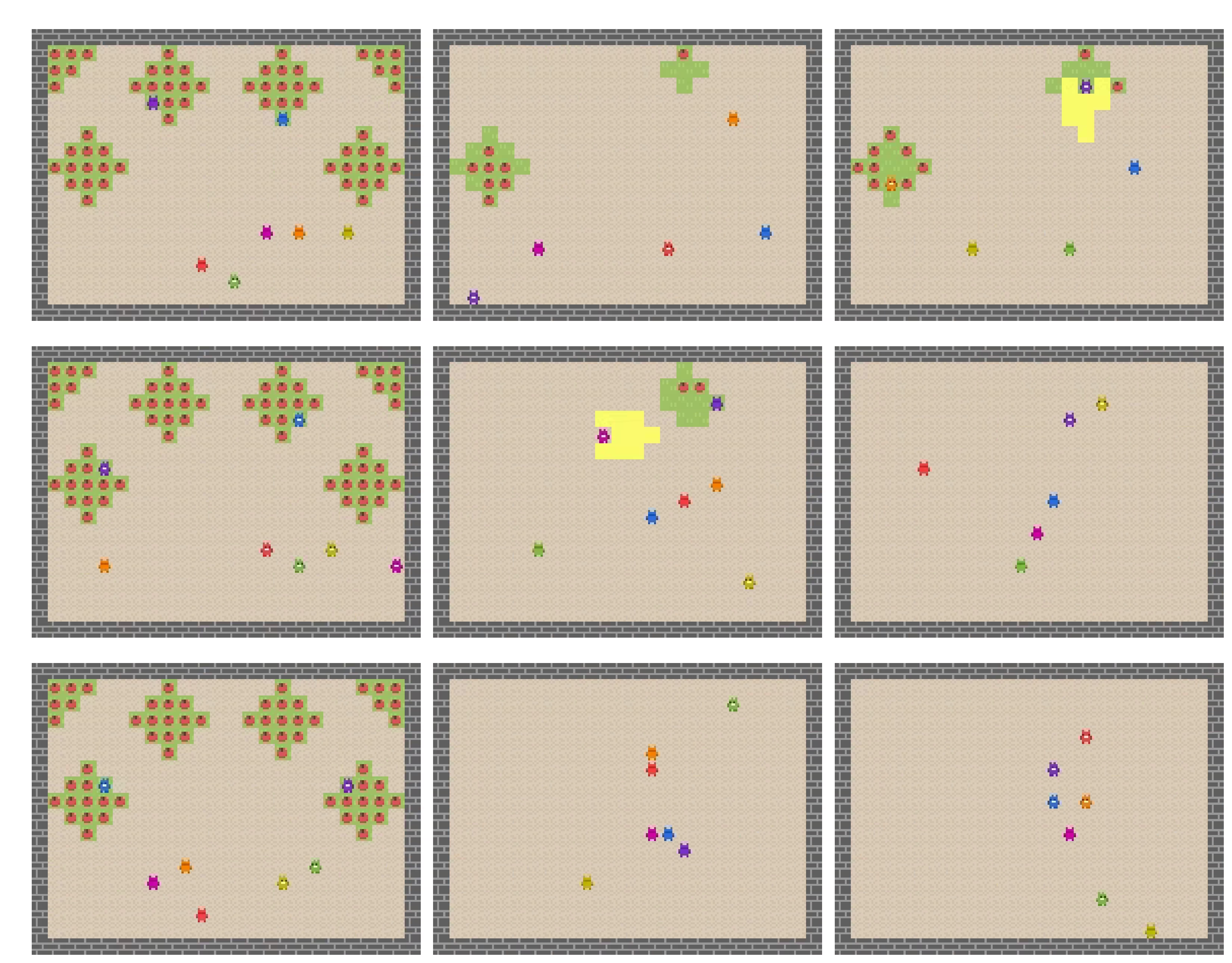
Frames of evaluation trajectories for different algorithms. Qualitatively, we demonstrate that Proximal Advantage Alignment (AdAlign, top) also outperforms naïve PPO (ppo) and PPO with summed rewards [next two rows]. The evaluation trajectories show how AdAlign agents are able to maintain a bigger number of apple bushes from extinction (2) for a longer time that either ppo or ppo p. Note that in the Commons Harvest evaluation two exploiter agents, green and yellow, play against a focal population of 5 copies of the evaluated algorithm.
I find this generally a mildly hopeful message for understanding and generating cooperation in general. Nation-states and businesses and other such entities all have a kind of learning awareness that we might model as “opponent-shaping”. Insofar as their interactions are approximately symmetric and the other assumptions are satisfied (consistency over time, etc) we can hope that nation-states might be able to achieve positive interactions in pairwise interactions.
Although, that said, with Actor-critic methods and small gradient updates it might take a few million interactions to learn the cooperating policies, so you don’t want to rely this in the real world, necessarily.
There is a more reassuring message here though: The strategic calculus of peer agents can potentially produce stable cooperation. The “arms race” of “I’m modelling you modelling me…” appears to be short; the original LOLA paper (Jakob Foerster, Chen, et al. 2018) found that a 2nd-order agent gained no significant advantage over a 1st-order one in self-play. We can interpret this in terms of strategic logic as follows:
- The cost of escalation is immense.
- The risk of effective retaliation is high.
- The probability of gaining a lasting, decisive edge is low.
The rational course of action is therefore not to attempt domination, but to secure a stable, predictable outcome. This leads to a form of AI Diplomacy, where the most stable result is a “Mutually Assured Shaping” equilibrium.
6.2 Asymmetric capabilities: Are humans opponent shapers, empirically?
Sometimes? Maybe? It seems like we can be when we work hard at it. But there is evidence that we ain’t good at being such shapers in the lab.
The Advantage Alignment paper admits asymmetric capabilities in its agents, but does not analyse such configurations in any depth. AFAIK, no one has tested Opponent Shaping policies against human by that name. However, we do have a paper which comes within spitting distance of it. The work by Dezfouli, Nock, and Dayan (2020) trains RL agents to control “surrogate” humans, since real humans are not amenable to running millions of training iterations.9 They instead set up some trials with human in a lab setting, and trained an RNN to ape human learning in various “choose the button” experiments. This infinitely patient RNN will subject itself to a punishing round of RL updates.
The goal of that paper is to learn to train RL agents to steer the humans with which they interact. The remarkable result of that paper is that RL policies learned on the surrogate humans transfer back to real humans. The adversary in those settings was highly effective at guiding human behaviour and developed non-intuitive strategies, such as strategically “burning” rewards to hide its manipulative intent.10
Against a sufficiently powerful RL agent, humans can be modelled as weaker learners, for one of several reasons.
- Modelling Capability: An AI can leverage vast neural architectures to create a high-fidelity behavioural model of a human, whereas a human’s mental model of the AI will be far simpler.
- Computational Effort: An AI can run millions of simulated interactions against its model to discover non-intuitive, effective policies. A human cannot, and often lacks the time or enthusiasm to consciously model every instance of digital operant conditioning they face daily.
- Interaction History: While the formalism only requires interaction data, an AI can process and find patterns in a vast history of interactions far more effectively than a human can.
The Dezfouli, Nock, and Dayan (2020) experiment demonstrated that this asymmetry could be readily exploited. One is that the asymmetric shaping capability is not necessarily mutually beneficial. Trained to exploit the naïve learner, this policy can find beneficial or indeed exploitative equilibria. A MAX adversary with a selfish objective learned to build and betray trust for profit, while a FAIR adversary with a prosocial objective successfully guided human players toward equitable outcomes. I don’t want to push the results of that paper too far here, not until I’ve done it over in an opponent-shaping framework for real. However we should not expect Opponent-shaping agents to be less effective than the naïve algorithm of Dezfouli, Nock, and Dayan (2020) at shaping the behaviour of humans.
The implications in that case are troubling both for humans in particular, and asymmetric interactions in general.
6.3 Unknown capabilities
OK, we did equally-capable agents, which leads to a virtuous outcome, and asymmetric agents which leads to a potentially exploitative outcome.
There is another case of interest, which is when it is ambiguous what the capabilities of two opponents are. This is probably dangerous. A catastrophic failure mode could arise if one agent miscalculates its advantage and attempts an exploitative strategy against an opponent it falsely believes to be significantly weaker, triggering a costly, destructive conflict. This creates a perverse incentive for strategic sandbagging, where it may be rational for an agent to misrepresent its capabilities as weaker than they are, luring a near-peer into a devastatingly misjudged escalation. True stability, therefore, may depend not just on raw capability, but on the ability of powerful agents to credibly signal their strength and avoid such miscalculations.
6.4 Scaling Opponent Shaping to many agents
OK, we have some mild hope about cooperation in adversarial settings in this model.
Let us leaven that optimism with qualms about scalability. This mechanism of implicit, pairwise reciprocity will face problems scaling up. We can get surprisingly good cooperation from this method, but I would be surprised if it were sufficient for all kinds of multipolar coordination.
Even in a setting such as no-online learning where the training cost for each of our \(N\) per-agent is a manageable \(\mathcal{O}(N)\) and execution is constant (i.e. we are not learning from additional experience “in the wild”), the sample complexity—the total amount of experience needed to learn effective reciprocity with all other agents—grows significantly. Furthermore, the communication overhead (i.e. interaction history) required to maintain these pairwise relationships we can imagine becoming a bottleneck for complicated interactions.11 We suspect this becomes intractable for coordinating large groups.12
Even with linear training-time scaling, sample inefficiency and coordination overhead likely swamp pairwise reciprocity once \(N\) grows large; this, rather than per-step compute, motivates institutions—laws, markets, social norms—that supply cheap global coordination. These are mechanisms of cooperative game theory, designed to overcome the scaling limits of pairwise reciprocity by establishing explicit, enforceable rules and shared infrastructure.
6.5 Noisy observation of partner intent
The Randomized Uncertain Social Preferences (RUSP) framework (Baker 2020) solves this by training agents across a distribution of prosocial weights, where each agent only gets a noisy observation of its own weights and no information about others’. At each episode start, we sample a reward-transformation matrix \(W\), where \(W_{ij}\) is the weight agent \(i\) puts on agent \(j\)’s reward, then have agent \(i\)’s shaped reward be \(\sum_j W_{ij} r_j\). Each agent observes only a noisy version of its own row (so it isn’t sure how much it should care about each partner), and nothing about other agents’ rows (so it can’t tell which partners care about it). Training is across the whole distribution of \(W\)s, not a single fixed one.
Because partner intent isn’t observable, the only way an agent can do well in expectation is to read intent from behaviour — cooperate cautiously, escalate cooperation when reciprocated, punish when defected against. The reported emergent phenomena are: direct reciprocity (tit-for-tat-ish responses to recent behaviour), indirect reputation tracking (treating an agent based on how it treated third parties), and stable in-episode team formation (subsets of agents settling into cooperative pairs while the rest go it alone). None of these are programmed in; they are policies that generalize across the \(W\)-distribution. Unlike fixed-prosocial-weights training, the policies reportedly transfer to held-out partner mixes without retraining.
7 Takeaways: Grounding strategic risk, and other uses for this formalism
The strategic landscape of AGI is often discussed in terms of intuitive but sometimes imprecise concepts. We talk about treacherous turns, manipulation, and collusion without always having a clear, mechanistic model of how these behaviors would be learned or executed. The primary value of the opponent shaping framework is that it provides precisely this: a minimal, tractable, and empirically testable formalism for grounding these intuitions, and some logical next experiments to perform.
The key takeaways are not the risks themselves—which are already in the zeitgeist—but how opponent shaping allows us to model them with new clarity.
7.1 From “Manipulation” to Computable Asymmetry.
The risk of an AI manipulating its human operators is a core safety concern. Opponent shaping translates this abstract fear of being ‘reward hacked’ (i.e., steered into preferences that benefits the AI at the human’s expense) into a concrete, measurable quantity. The opponent-shaping framework gives us two ‘knobs’ to model this asymmetry: the explicit shaping parameter (\(\beta\)), which controls how much an agent cares about influencing the opponent, and the implicit fidelity of its opponent model. An agent with a superior ability to estimate its opponent’s advantage (\(A^{\text{opponent}}\)) can achieve more effective shaping, even with the same \(\beta\). This turns the abstract fear of manipulation into a testable model of informational and computational asymmetry. From here we can re-examine proof-of-concept papers like Dezfouli, Nock, and Dayan (2020) with more tunable theory of mind. What do the strategies of RL agents, armed with a basic behavioural model, look like as we crank up the computational asymmetries? Opponent shaping allows us to start modelling asymmetry in terms of a learnable policies.
7.2 Treacherous turns
The concept of a treacherous turn—an AI behaving cooperatively during training only to defect upon deployment—is often framed as a problem of deception. Opponent shaping is an interesting way to model this, as the optimal long-term policy for a self-interested agent with a long time horizon (\(\gamma \to 1\)). The investment phase of building trust by rewarding a naïve opponent is simply the early part of a single, coherent strategy whose terminal phase is exploitation. This temporal logic is captured by the alignment term, \(\beta\gamma(\sum_{k<t}...\ )A^{\text{opponent}}_t\), in the effective advantage update. This allows us to analyse the conditions (e.g., discount factors, observability) under which a treacherous turn becomes the default, profit-maximizing strategy, although let us file that under “future work” for now.
7.3 AI Diplomacy
We speculate about how powerful AIs might interact, using analogies from international relations. The opponent shaping literature, particularly the finding that the 2nd-order vs 1st-order LOLA arms race is short, provides a formal basis for AI-AI stability. It suggests that a “Mutually Assured Shaping” equilibrium is a likely outcome for peer agents. This is not based on altruism, but on the cold calculus that the expected return from attempting to dominate a fellow shaper is negative. This provides a mechanistic model for deterrence that doesn’t rely on analogy. It also allows us some interesting hypotheses, for example: a catastrophic conflict is most likely not from pure malice, but from a miscalculation of capabilities in a near-peer scenario, leading to a failed attempt at exploitation.
7.4 From Scalable Oversight to Institutional Design
The problem of managing a large population of AIs is often framed as a need for ‘scalable oversight.’ The quadratic complexity of pairwise opponent shaping gives this a computational justification. It formally demonstrates why pairwise reciprocity fails at scale and why designed institutions (mechanisms from cooperative game theory) are likely a computational necessity, at least in this competitive game-theory setting. It reframes the AI governance problem away from solely aligning individual agents and toward the distinct problem of designing the protocols, communication standards, and monitoring systems that constitute a safe multi-agent environment.
8 Next Steps
This has been a great learning exercise for me, and help me crystallise many half-formed ideas. My next steps are to apply this formalism to model specific strategic scenarios, such as the treacherous turn or multi-agent institutional design. Feel free to reach out if you want to take it somewhere.
9 Acknowledgements
- Juan Duque graciously answered my questions about the Advantage Alignment.
- Seijin Kobayashi spent substantial time helping me understand Meulemans et al. (2024).
- Gemini Pro 2.5 expanded my dot points into drafts which I then completely rewrote because its prose is painful. It was much more effective at critiquing my document structure though — you can thank it for the appendices.
- ChatGPT o3 checked my mathematics
10 Appendix: Game theory
Our setting is classical non-cooperative game theory, as opposed to the cooperative flavour (the technical term is “General-Sum Markov Games”).13 That is to say, we are modelling the situation where players cannot choose whether to play the game, or how to set the rules, or create commitments; Instead, they are handed the game, and must play the game as given.
For the current purposes, we care about “mixed” strategy games, which is the game-theoretic term for stochastic games, wherein players can randomize their actions.
A one-shot game is a classical game where players choose their actions simultaneously and then receive payoffs.
Players A finite set \(N=\{1,2,\dots,n\}\).
Actions Each player \(i\) has a finite action set \(A_i\). A joint action is \(\mathbf a=(a_1,\dots,a_n)\in A_1\times\cdots\times A_n\).
Payoffs When the joint action \(\mathbf a\) is played, player \(i\) receives utility
\[ u_i(\mathbf a)\;=\;u_i(a_1,\dots,a_n)\;\in\;\mathbb{R}. \]
This is the bit you write as a table when you are in a two-player game. So for example, in the Prisoner’s Dilemma, the payoffs are
Dan: C Dan: D Alice: C (R,R) (S,T) Alice: D (T,S) (P,P) where \(R\) is the reward for cooperating, \(T\) is the temptation to defect, \(S\) is the sucker’s payoff, and \(P\) is the punishment for mutual defection. Conventionally \(T> R > P > S\) and \(2R > T + S\).
Strategies
A mixed strategy for player \(i\) is a probability distribution over their actions. (While deterministic “pure” strategies are a special case, our focus is on these stochastic strategies).
\[ \sigma_i:A_i\;\to\;[0,1], \quad \sum_{a_i\in A_i}\sigma_i(a_i)=1. \]
We call the set of action probabilities for all players the profile, \(\sigma=(\sigma_1,\dots,\sigma_n)\). Each player \(i\) samples
\[ a_i\;\sim\;\sigma_i(\cdot). \]
Each draw is independent across players by assumption. Hence, the joint action \(\mathbf a=(a_1,\dots,a_n)\) is a random vector whose probability mass is
\[ \Pr\bigl(a_1,\dots,a_n\bigr) = \prod_{i=1}^n \sigma_i(a_i). \]
Expected Utility Player \(i\) cares about their expected utility over this mass function,
\[ u_i(\sigma) = \mathbb{E}_{a_1\sim\sigma_1,\;\dots,\;a_n\sim\sigma_n} \bigl[u_i(a_1,\dots,a_n)\bigr] \;=\; \sum_{(a_1,\dots,a_n)} \Bigl(\underbrace{\prod_{j=1}^n \sigma_j(a_j)}_{\Pr(a_1,\dots,a_n)}\Bigr) \,u_i(a_1,\dots,a_n). \]
We formalize which profiles actually make sense (i.e. are rational) via the (mixed-strategy) Nash equilibrium.
Suppose I am agent \(i\). Fix everyone else’s profile \(\sigma^*_{-i}\). My strategy \(\sigma_i\) is a best response if \[ u_i(\sigma_i,\sigma^*_{-i}) \;=\; \max_{\tau_i\in\Delta(A_i)} u_i(\tau_i,\sigma^*_{-i}). \]
A profile \(\sigma^*=(\sigma^*_1,\dots,\sigma^*_n)\) is a Nash equilibrium if each player’s strategy \(\sigma^*_i\) is a best response to the other players’ strategies \(\sigma^*_{-i}\), which implies that no single player can unilaterally tweak their probabilities and raise their expected payoff.
Nash equilibria quantify the incentive to unilaterally deviate from a strategy; if it’s a Nash equilibrium, then no player has such an incentive. So: double defect in the classic prisoner’s dilemma is famously a Nash equilibrium in the one-shot game. Buuut…
10.1 Iterated Games and “Good” Equilibria
Once we let players interact repeatedly, the dynamics are more interesting, because we are in the realm of the folk theorem. Loosely this tells us that anything above the minmax payoff can be sustained as a Nash equilibrium in the iterated game, and many of these equilibria are “good” in the sense that they are Pareto-superior to the min-max fallback.
We could at this juncture go deep on formalizing these ideas; define games, set a discount factor \(\delta\in(0,1)\), devise computational complexity results for finding Nash equilibria etc… Let’s keep it intuitive for the moment. In an iterated game (played over, say, an infinite horizon with a discount factor \(\delta\in(0,1)\)), players’ histories matter, opening the door to strategies like reciprocity and punishment.
10.2 Axelrod’s Tournaments and evolutionary games
Robert Axelrod ran computer tournaments to see which strategies thrive in an indefinite Prisoner’s Dilemma. The surprise winner was Tit-for-Tat: start with Cooperation, then mirror your opponent’s last move.
That work spawned a line of inquiry into “good” equilibria under noise, mistakes, and evolutionary selection. We now know that robust cooperation often requires a mix of generosity, clarity, and punish-but-pardon dynamics—far richer than any one-shot analysis could predict.
We can generalize also to ecological settings and explore the population dynamics of different strategies in a population of agents.
In all these traditional cases we formalise the choice of strategy without regard to considering how the agents can learn them; machine learning was not much of a thing when all these models were first developed. I won’t go down that classic path—because it is a sure-fire way to confuse machine-learning people— ML practitioners prefer not to go straight from “data” to “strategy” (with some implied “reasoning” in there) but rather to imagine how a strategy might be “learned”, since the learning from data rather than deducing from pure reason is the bit that pays the bills.
Even if you could represent it, solving for a Nash equilibrium in general-sum games is PPAD-complete (Yannakakis 2009), so nobody expects efficient global-optimum finding in the worst case.
So, if we want to make the game learnable, we need a model of learning to act. A natural model for such a problem (learning strategies while playing games) is, of course…
11 Appendix: Reinforcement learning
In broad strokes, RL is a formalization of precisely this kind of problem. Specifically, it tells us how to learn to take good actions in various circumstances by trying things out. Formally, RL models give us (descriptive/prescriptive) models for how we learn to make decisions in the world.
You could see my quick personal overview for a tutorial introduction to Reinforcement Learning if you needed to get up to speed but were time-strapped. If you have more time, I would recommend a proper tutorial. RL is big business and well-studied, and there are many fine resources which can instil a handsome grounding in the field.
11.1 Solipsistic RL
The base case in RL is essentially solipsistic: one agent versus the world. The classic exemplar that we all imprint in RL class upon is just such a case, the CartPole problem Figure 7. We’ll extend to less solipsistic interactions in a moment, but just to get the flavour of RL let’s think about CartPole for a moment.

From the perspective of the agent, the world in RL presents us with a Markov Decision Problem (MDP). Formally, an MDP is the tuple \((\mathcal{S},\mathcal{A},P,R,\gamma)\), where
- \(\mathcal{S}\) is the set of states,
- \(\mathcal{A}\) the set of actions,
- \(P(s' \mid s,a)\) the transition kernel,
- \(R(s,a)\) the (expected) immediate reward, and
- \(\gamma\in[0,1)\) the discount factor.
At each time step \(t\), the agent in state \(s_t\) picks an action \(a_t\), transitions to \(s_{t+1}\sim P(\cdot\mid s_t,a_t)\), and observes reward \(r_t=R(s_t,a_t)\). The learning objective is to find a policy \(\pi(a\mid s)\) that maximizes the expected return
\[ \mathbb{E}_{\pi}\Bigl[\sum_{t=0}^\infty \gamma^t\,r_t\Bigr]. \]
All of the RL methods we’ll discuss are ways to approximate or converge to that optimal policy in single- or multi-agent settings.
Without getting excessively technical the key point is that the MDP assumes the world is Markovian, which means that the next state \(s_{t+1}\) depends only on the current state \(s_t\) and action \(a_t\), not on the history of previous states or actions.14 The upshot is that there are many historical details we can ignore; the past is relevant only to the extent that it affects the current state, and the current state is all we need to make a decision.
So in the CartPole example, the agent only needs to know the current state of the cart and pole (position, velocity, angle, and angular velocity) to decide how to act. How we got to the current precarious state of pole-balancing is irrelevant.
11.2 Advantage
The advantage function is a concept designed to isolate the benefit of a particular action. It can be thought of as the natural variance-reduced signal that connects value estimation to policy improvement.
To unpack that, we need two concepts:
State-Value \(V^\pi(s)\): The expected future reward if you start in state \(s\) and follow your policy \(\pi\) from then on. Think of it as “how good is it to be in this situation?” \[ V^\pi(s)=\mathbb{E}\Bigl[\sum_{t=0}^\infty\gamma^t\,r_t\;\Bigm|\;s_0=s\Bigr]. \]
Action-Value \(Q^\pi(s,a)\): The expected future reward if you start in \(s\), take a specific action \(a\), and then follow your policy \(\pi\). Think of it as “how good is it to take this specific action in this situation”? \[ Q^\pi(s,a) =\mathbb{E}\Bigl[r_0 + \gamma\,V^\pi(s_1)\;\Bigm|\;s_0=s,\,a_0=a\Bigr]. \]
Smashing them together we get the Advantage Function \(A(s,a)\), the difference between the two:
\[ A(s,a) = Q(s,a) - V(s). \]
It isolates the value of an action by answering the question: “How much better or worse was taking action \(a\) compared to the average value of this state?”
AFAICT, it serves two purposes: variance reduction and better attribution.
1. Variance Reduction: A basic policy gradient update learns by scaling the gradient of an action by the total sampled return (\(R_t\)). \[ \nabla_\theta J \propto \mathbb{E}\Bigl[\sum_t\!\nabla_\theta\log\pi_\theta(a_t\!\mid s_t)\,\times\,\underbrace{R_t}_{\text{sampled return}}\Bigr]. \] The problem is that raw returns are famously noisy. By subtracting a baseline that doesn’t depend on the action, we can reduce this variance without introducing bias. The state-value \(V(s_t)\) is a natural choice. The resulting term, \(R_t - V(s_t)\), is an estimate of the advantage, \(A(s_t,a_t)\). This gives us the canonical advantage-actor-critic update, which is much more stable: \[ \nabla_\theta J \;\approx\; \mathbb{E}\Bigl[\nabla_\theta\log\pi_\theta(a_t\!\mid s_t)\;A(s_t,a_t)\Bigr]. \]
2. Better Attribution: The advantage function disentangles two questions that are otherwise conflated:
- How good was this state overall? → This is answered by \(V(s)\).
- How good was this specific action in that state? → This is answered by \(A(s,a)\).
If an action is merely average (\(A(s,a) \approx 0\)), we don’t need to push the policy toward or away from it, even if the overall outcome was great. Only actions that are significantly better or worse than average should drive learning, and the advantage function isolates exactly that signal.
11.3 How Agents Learn Values
We’ve defined the state-value function \(V^\pi(s)\) as the expected future reward. But how does an agent actually calculate this value while playing a game, especially when it doesn’t know the rules (\(P\) and \(R\)) in advance? It has to learn from experience.
One simple approach is the basic Monte Carlo method:
- Play an entire episode from start to finish.
- For every state
svisited, record the actual total future reward (\(G_t\)) that was received from that point onward. - Average these returns over many episodes to estimate \(V(s)\).
This works in principle, but it’s slow and inefficient. You have to wait until the very end of an episode to get a single data point for learning.
A more effective and common approach is Temporal-Difference (TD) learning, which updates estimates without waiting for an episode to end. Instead of waiting for the final outcome, we update our estimate based on another, slightly later estimate. We learn from the difference between our guess at one time step and our guess at the next. You might be wondering when this converges; AFAICT the answer is “sometimes”.
Here’s how it works for learning the state-value function, \(V(s)\):
- At time
t, the agent is in state \(s_t\). It has a current estimate for its value, \(V(s_t)\). - It takes an action \(a_t\), receives a reward \(r_t\), and lands in a new state \(s_{t+1}\).
- It then looks at its own estimate for the value of the next state, \(V(s_{t+1})\).
- It computes a TD Target: this is a new, more informed estimate of what \(V(s_t)\) should have been. It’s simply the immediate reward plus the discounted value of the next state: \[ \text{TD Target} = r_t + \gamma V(s_{t+1}) \]
- It then computes the TD Error (also called the surprise): the difference between this better target and its original estimate. \[ \text{TD Error} = (r_t + \gamma V(s_{t+1})) - V(s_t) \]
- Finally, it nudges its original estimate in the direction of the error: \[ V(s_t) \leftarrow V(s_t) + \alpha \times (\text{TD Error}) \] where \(\alpha\) is a small learning rate.
This process of “bootstrapping”—updating our value estimate for a state using the estimated value of subsequent states—is the engine behind most modern reinforcement learning. When the main text says an agent “fits a critic by TD,” it means it is running exactly this update process to continuously refine its estimate of a value function (\(V\) or \(Q\)) using the stream of rewards it observes during the game.
12 Appendix: Multi-agent Reinforcement Learning

Multi-agent RL combines game theory and reinforcement learning, asking “What if the environment is not a pole-balancing cart, but another agent, with learning algorithms of its own?” This case was made famous by AlphaGo/AlphaZero: Systems that learn to play against (or with) each other.
In this setting the world is not generally Markovian, in the sense that while we might be able to infer physical states, we know that the unobserved mental states of our opponent matter too. Once we let everyone learn at the same time, the “environment” that we represent to each other becomes both partially-observed and non-stationary: as I learn, so does everyone else. Thus our behaviour changes over time, and the optimal response to that behaviour can change too. Classical convergence guarantees break down because the transition kernel \(P(s' \mid s,a)\) now depends on how all the other learners’ policies evolve.
Littman (1994) formalized it first, the idea of using reinforcement learning to play games. The argument seems to have two parts:
- If we hold fixed all other players’ policies, then the game reduces to a Markov decision process (MDP) and we can use reinforcement learning to learn a policy for that MDP. It will learn the best response to the other players’ policies.
- If we do not hold fixed the opponent’s policies, then we are now playing a game in the game-theoretic sense, and we can try to generalize RL to find a Nash equilibrium of the game. Littman introduces a Minimax-Q update which looks neat but I am not sure we need it here. Hold that thought.
On top of that, the joint action space grows exponentially with the number of agents \(n\), so naïvely estimating a full value function \(Q(s, a^{\textrm{Dan}}, a^{\textrm{Alice}}, \dots, a^n)\) quickly becomes intractable.
The challenge becomes a partial observability problem: if an agent could observe its opponent’s internal state (e.g., its policy parameters or value estimates), the optimal response would be much easier to compute.
Could I estimate that opponent’s beliefs from their actions? That feels unattainable — naïvely it would require each agent to be as complicated as all the other agents put together, including itself. What, we might wonder, is a sufficiently sophisticated model to capture the opponent’s beliefs enough to respond to them well? Do I need a full-blown theory of mind? Great question, self!
We have arrived at one of the main ideas of multi-agent reinforcement learning, from which we will deduce opponent shaping, back in the main body of the text.
The natural approach expands the model slightly. We start with two agents. In a two-player Markov game (or general \(n\)-player extension), each agent \(i\) has a policy \(\pi_i(a\mid s;\theta_i)\) parameterized by \(\theta_i\). Let \(\tau=(s_0,a_0,b_0,s_1,a_1,b_1,\dots)\) denote a trajectory generated by the joint policy \(\pi^{\textrm{Dan}},\pi^{\textrm{Alice}}\). We write agent \(i\)’s immediate reward at time \(t\) as \(r^i_t = r^i(s_t,a_t,b_t)\), and discount future payoffs by \(\gamma\in[0,1)\).
Joint value functions. Agent 1’s expected return under \((\theta^{\textrm{Dan}},\theta^{\textrm{Alice}})\) is
\[ V^{\textrm{Dan}}(\theta^{\textrm{Dan}},\theta^{\textrm{Alice}}) \;=\; \mathbb{E}_{\tau\sim\pi^{\textrm{Dan}},\pi^{\textrm{Alice}}} \Bigl[\sum_{t=0}^\infty \gamma^t\,r^{\textrm{Dan}}_t\Bigr], \]
and analogously
\[ V^{\textrm{Alice}}(\theta^{\textrm{Dan}},\theta^{\textrm{Alice}}) \;=\; \mathbb{E}_{\tau\sim\pi^{\textrm{Dan}},\pi^{\textrm{Alice}}} \Bigl[\sum_{t=0}^\infty \gamma^t\,r^{\textrm{Alice}}_t\Bigr]. \]
Action-value (“Q”) and advantage functions. We define the joint action-value for agent 1 as
\[ Q^{\textrm{Dan}}(s,a,b) \;=\; \mathbb{E} \Bigl[r^{\textrm{Dan}}_0 + \gamma\,V^{\textrm{Dan}}(\theta^{\textrm{Dan}},\theta^{\textrm{Alice}})\,\bigm|\,s_0=s,\,a_0=a,\,b_0=b\Bigr], \]
and its corresponding advantage \(A^{\textrm{Dan}}(s,a,b) = Q^{\textrm{Dan}}(s,a,b) - V^{\textrm{Dan}}(\theta^{\textrm{Dan}},\theta^{\textrm{Alice}}).\) Agent 2’s \(Q^{\textrm{Alice}}\) and \(A^{\textrm{Alice}}\) are defined analogously based on its own rewards, \(r^{\textrm{Alice}}\).
These definitions let us write each player’s policy-gradient in standard REINFORCE (or actor–critic) form, and track how one agent’s update depends on both \(\theta^{\textrm{Dan}}\) and \(\theta^{\textrm{Alice}}\).
13 Appendix: LOLA cross gradient in IPD
13.1 The Cross-Hessian Term
\(\Large\partial_{\theta^{\mathrm{Dan}}}\partial_{\theta^{\mathrm{Alice}}}V^{\mathrm{Dan}}\)
Write Dan’s stage-game value as
\[ V^{\mathrm{Dan}}(p_{\textrm{Dan}},p_{\textrm{Alice}})= (R-S-T+P)\,p_{\textrm{Dan}}p_{\textrm{Alice}} +(S-P)\,p_{\textrm{Dan}} +(T-P)\,p_{\textrm{Alice}} +P . \]
With the numbers above \(R-S-T+P=-1\). A single derivative w.r.t. \(p_{\textrm{Alice}}\) gives
\[ \frac{\partial V^{\mathrm{Dan}}}{\partial p_{\textrm{Alice}}}= (R-S-T+P)\,p_{\textrm{Dan}}+(T-P)=4-p_{\textrm{Dan}} . \]
Convert to \(\theta\)-space using \(\partial p/\partial\theta=p(1-p)\):
\[ \frac{\partial V^{\mathrm{Dan}}}{\partial\theta^{\mathrm{Alice}}} =(4-p_{\textrm{Dan}})\,p_{\textrm{Alice}}(1-p_{\textrm{Alice}}). \]
Now differentiate that w.r.t. \(\theta^{\mathrm{Dan}}\):
\[ \boxed{\; \frac{\partial^{2}V^{\mathrm{Dan}}}{\partial\theta^{\mathrm{Dan}}\partial\theta^{\mathrm{Alice}}} =-\,p_{\textrm{Dan}}(1-p_{\textrm{Dan}})\,p_{\textrm{Alice}}(1-p_{\textrm{Alice}}) \;} . \]
13.2 Alice’s gradient
\(\large\partial_{\theta^{\mathrm{Alice}}}V^{\mathrm{Alice}}\)
Symmetry gives
\[ \frac{\partial V^{\mathrm{Alice}}}{\partial p_{\textrm{Alice}}}= (R-S-T+P)\,p_{\textrm{Dan}}+(S-P)=-(1+p_{\textrm{Dan}}), \]
so
\[ \boxed{\; \frac{\partial V^{\mathrm{Alice}}}{\partial\theta^{\mathrm{Alice}}} =-(1+p_{\textrm{Dan}})\,p_{\textrm{Alice}}(1-p_{\textrm{Alice}}) \;} . \]
13.3 The LOLA cross term
LOLA adds
\[ \beta\; \underbrace{\frac{\partial^{2}V^{\mathrm{Dan}}}{\partial\theta^{\mathrm{Dan}}\partial\theta^{\mathrm{Alice}}}} _{-\;p_{\textrm{Dan}}(1-p_{\textrm{Dan}})\,p_{\textrm{Alice}}(1-p_{\textrm{Alice}})} \; \underbrace{\frac{\partial V^{\mathrm{Alice}}}{\partial\theta^{\mathrm{Alice}}}} _{-(1+p_{\textrm{Dan}})\,p_{\textrm{Alice}}(1-p_{\textrm{Alice}})} \]
to my ordinary policy-gradient, giving
\[ \boxed{\; \text{cross-term}=\; \beta\;p_{\textrm{Dan}}(1-p_{\textrm{Dan}})\,[p_{\textrm{Alice}}(1-p_{\textrm{Alice}})]^{2}\,(1+p_{\textrm{Dan}}) \;} . \]
13.4 plug it in
We check at the centre point \(p_{\textrm{Dan}}=p_{\textrm{Alice}}=\tfrac12\):
\[ p_i(1-p_i)=0.25. \qquad \text{cross-term}= \beta\;(0.5)(0.25)^{2}(1.5) = \beta\times0.0234375. \]
The selfish gradient there is \(-0.375\); consequently the very first update switches sign only when
\[ \beta_{\mathrm{flip}}=\frac{0.375}{0.0234375}\approx16. \]
13.5 Appendix: Spite
The advantage-product term \(\Bigl(\sum_{k<t}\gamma^{t-k}A^{\textrm{Dan}}_k\Bigr)\,A^{\textrm{Alice}}_t\) creates intuitive dynamics for cooperation (positive * positive) and retaliation (positive * negative). The case where my cumulative past advantage and Alice’s current advantage are both negative leads to a counter-intuitive (for me at least) result.
Consider a situation where:
- My cumulative past advantage is negative: The history of the game has been bad for me.
- Alice’s current advantage is also negative: The action she just took was worse for her than her average.
In this scenario, the alignment term is the product of two negatives, which is positive. This seems to be a peculiar learning signal. My own direct experience (my advantage, \(A^{\textrm{Dan}}_t\)) tells me the last action was bad and should be suppressed. However, the alignment term provides a positive push, working against my selfish gradient.
The effective advantage becomes: \[ A^*_t = \underbrace{A^{\textrm{Dan}}_t}_{\text{Negative}} + \underbrace{\text{Alignment Term}}_{\text{Positive}} \]
If the positive alignment term is strong enough to overcome my own negative advantage, I will learn to increase the probability of an action that was part of a mutually harmful outcome. This is a potential failure mode of the simple alignment logic, where agents can get stuck reinforcing mutual misery—a dynamic that appears “spiteful” as it perpetuates harm for both parties.
The authors of Advantage Alignment (Duque et al. 2025) were aware of this potential pathology and explored it in their ablations (see Figure 7 in their paper).
But also, I don’t quite know what to make of it; it presumably arises in LOLA as well.
14 Incoming
Meulemans et al. (2024):
Promising recent work has shown that in certain tasks cooperation can be established between “learning-aware” agents who model the learning dynamics of each other. Here, we present the first unbiased, higher-derivative-free policy gradient algorithm for learning-aware reinforcement learning, which takes into account that other agents are themselves learning through trial and error based on multiple noisy trials. We then leverage efficient sequence models to condition behaviour on long observation histories that contain traces of the learning dynamics of other agents. Training long-context policies with our algorithm leads to cooperative behaviour and high returns on standard social dilemmas, including a challenging environment where temporally-extended action coordination is required.
The Causal Incentives Working Group generalizes game theory in several interesting ways that are relevant to our models.
Calvano et al. (2020) finds collusion and punishment in pricing games with RL agents despite no explicit communication or other modeling. How does that work?
Weis et al. (2026): Google finds that AI agents learn to cooperate when trained against unpredictable opponents
15 References
Footnotes
The additional condition \(2R > T + S\) is also common, ensuring that taking turns defecting isn’t better than consistently cooperating.↩︎
I am committing an act of machine-learning chauvinism here for the sake of simplicity. If you include evolutionary learning as a learning algorithm, then much effort has been spent on modelling strategies in evolutionary game theory, starting with the notion of Evolutionarily Stable strategies (Smith and Price 1973).↩︎
The name itself is something of a misnomer, suggesting pure conflict in that term “Opponent”, but it applies equally to games where a cooperative outcome is attainable.↩︎
The open-weight setting brings us to Open Source Game Theory Critch, Dennis, and Russell (2022), which is a distinct, though related, field.↩︎
The full definitions can be found in the Advantage appendix.↩︎
There are many variants of LOLA that we are not expanding upon here; AFAICT Advantage Alignment is the first one to be substantially more comprehensible and practical, but I could have missed some.↩︎
Duque et al. (2025) prove the equivalence to LOLA under on-policy sampling. For off-policy or offline data you must apply importance weighting (e.g. V-trace, Retrace) or the gradient is biased.↩︎
implementation in the form of a solution to anthropogenic climate change is left as an exercise for the reader↩︎
This Dezfouli paper is IMO straight 🔥; I don’t know why it isn’t more frequently discussed.↩︎
This is a fascinating result from the paper: to prevent the human from realizing they were being manipulated into a low-reward action, the AI would sometimes forego a high reward for itself on a different action, obscuring the pattern and keeping the human compliant for longer.↩︎
In the wild, agents are likely not independent, but that is a whole other story, for a more elaborate formalism.↩︎
There is another sense in which we expect this not to scale to massively multiplayer games such as the famed multi-polar-trap because the reward signal is too dilute, but that is a matter for a future post. Maybe start with the mean-field formulation of Yang et al. (2018).↩︎
You could read my notes on game theory and then Iterated and evolutionary game theory for a tutorial introduction to iterated game theory. Better yet, read a more authoritative tutorial from elsewhere on the internet.↩︎
We still allow the worlds to be random, but the randomness too is independent of the history of the process. We can also extend this with “partially observable MDPs” (POMDPs) where the agent only sees a partial observation \(o_t\) of the state \(s_t\). That is almost always done in practice AFAICT but doesn’t add much to the discussion here, so I won’t go into it. See e.g. Kaelbling, Littman, and Cassandra (1998) for a good overview.↩︎