When a journal thins review instead of rationing it, the collapse is a cliff
2026-09-14
A variant of the AI-drafting journal model in which the journal reviews every submission less carefully rather than skipping some, and the smooth decline becomes a fold with hysteresis.
academe
collective knowledge
economics
how do science
incentive mechanisms
institutions
machine learning
Status: Draft, spun out of Should our journal publish AI-drafted manuscripts?, whose model and parameters this post assumes. I’m not sure there is much in this; I just wanted to stop claude fussing about a neat emergence of catastrophe theory in an economic model, which is cool, but not relevant.
In the parent post I assumed that the journal holds the review depth \(h\) fixed and rations the coverage proportion \(r\) by skipping some papers. The failure in such a setting is not too badly behaved, in that the equilibrium is unique, welfare falls continuously in AI capability \(a\), and a marginal improvement — a little more budget, a slightly better classifier — buys a proportionate marginal repair.
We could contrariwise imagine the journal absorbs a growing volume of submissions by reviewing all of them less carefully: coverage is fixed \(r = 1\), and each manuscript gets \(e = R/N\) reviewer-hours instead of the fixed \(h\). That puts congestion “inside” the incentives: the return to substance is now scaled by the per-manuscript attention \(e\), so as review thins, even high-quality authors would stop investing in the substance of manuscripts, which frees more time for volume, which thins review further. That feedback loop produces weird, pathological behaviour, depending on the proportion of authors of type \(H\) and \(L\).
Code
import numpy as npimport matplotlib.pyplot as pltfrom livingthing.matplotlib_style import set_livingthing_styleset_livingthing_style()# Parameters of the parent post.P =dict(theta=1.0, s_L=0.30, sbar=0.50, t_min=0.05, f=0.50, T=1.0, lam=0.25, R=16.0, h=10.0, b=1.0)def logistic(x):return1.0/ (1.0+ np.exp(-np.clip(x, -60, 60)))
Code
T2 = np.geomspace(P["t_min"], 25.0, 600)def tH_dilute(e, delta, p=P):"""H's optimal substance time when acceptance depends on attention e.""" obj = logistic(e * (p["theta"] * np.sqrt(T2) - p["sbar"])) / (T2 + delta)return T2[int(np.argmax(obj))]def dilution_equilibria(a, p, n=600):"""All fixed points of e * N(e) = R in the dilution variant.""" delta = p["f"] / a nL = p["T"] / (p["t_min"] + delta)def load(e): tH = tH_dilute(e, delta, p)return p["lam"] * p["T"] / (tH + delta) + (1- p["lam"]) * nL es = np.geomspace(0.1, 50.0, n) g = np.array([e * load(e) - p["R"] for e in es]) roots = []for i inrange(n -1):if (g[i] <0) != (g[i +1] <0): lo, hi = es[i], es[i +1]for _ inrange(40): mid = np.sqrt(lo * hi)if ((mid * load(mid) - p["R"]) <0) == (g[i] <0): lo = midelse: hi = mid roots.append(np.sqrt(lo * hi))return rootsfold_a = np.concatenate([np.linspace(1.5, 3.1, 20), np.linspace(3.1, 3.7, 45), np.linspace(3.7, 8.0, 20)])fig, axes = plt.subplots(1, 2, figsize=(9.5, 3.4), sharey=True)for ax, lam inzip(axes, (0.25, 0.75)): p2 =dict(P, lam=lam)for a in fold_a:for e in dilution_equilibria(a, p2): ax.plot(a, e, "o", ms=3, color="#7f4c94") ax.set_xlabel("AI capability $a$") ax.set_title(f"$\\lambda = {lam}$")axes[0].set_ylabel("equilibrium attention $e$")fig.tight_layout()plt.show()
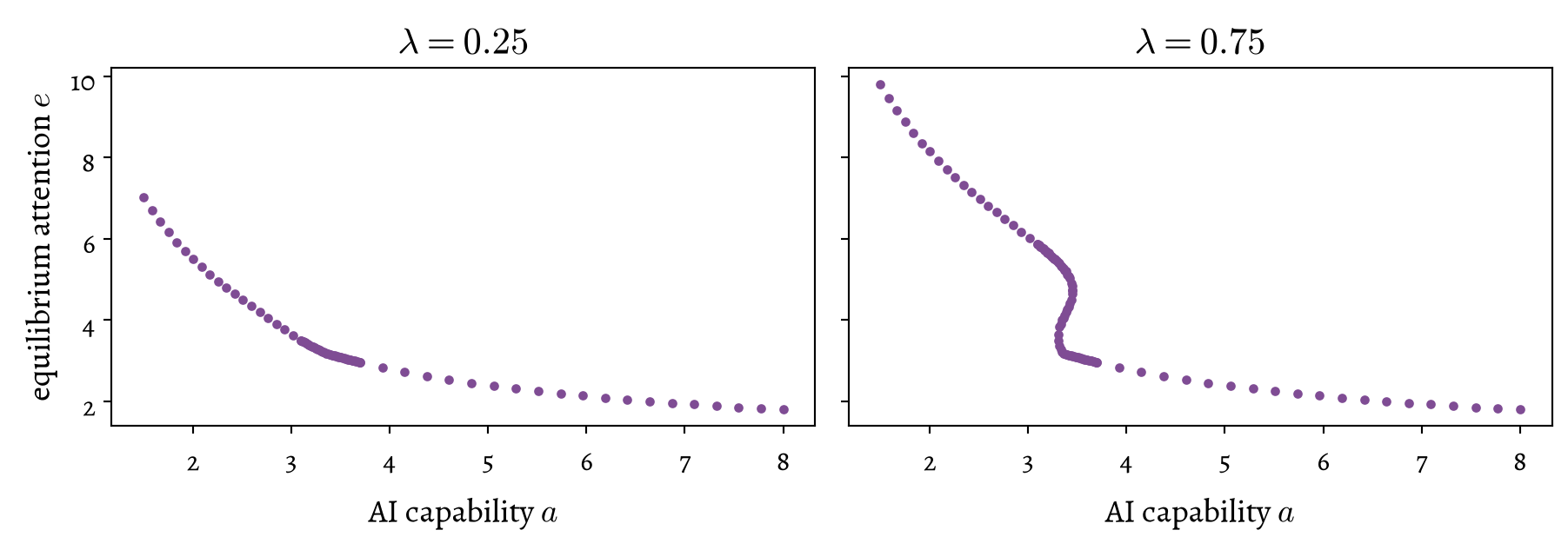
Figure 1: Equilibrium attention \(e\) at each capability \(a\), in the variant where the review depth \(h\) is spread across the whole queue, everything else as in the baseline. Left: at the baseline mix \(\lambda = 0.25\) the equilibrium is unique everywhere, so the decline is a slope. Right: at \(\lambda = 0.75\) a narrow range of \(a\) has three equilibria — a high-attention branch, a collapsed branch, and an unstable one between — so the decline is a cliff.
Figure 1 illustrates one case of each. At the baseline author mix, \(\lambda = 0.25\), the dilution variant also declines smoothly: one equilibrium at every \(a\). At \(\lambda = 0.75\) there is a narrow range of capability values, around \(a \approx 3.4\), in which three equilibria exist at once; the middle one is unstable, so in practice the journal is in one of two self-consistent states: careful review with restrained submission, or cursory review with a flood. Which state it ends up in depends on its history. Suppose the journal is in the careful state and \(a\) rises through this range. The journal stays careful, changing only a little — until, at the top of the range, the careful state stops being self-sustaining at all, and the journal falls to the flooded state in one step. The fall does not reverse: lower \(a\) back into the range and the journal stays flooded, because the flooded state is self-sustaining there too. Nobody can lower \(a\), but the model only sees \(a\) through the drafting cost \(\delta = f/a\), and a journal can raise that: a fee adds to the cost of every manuscript, and a ban above the slop authors’ threshold resets it to \(f\). Recovery means raising the effective cost of a manuscript well past the level at which the fall began, to where the flooded state itself stops existing, or else expanding the review budget \(R\) enough to move the fold. @Bartolucci2026Queue works this margin out properly in a queueing model: under load, reviewers rationally raise the risk threshold for checking AI output, cutting scrutiny when it matters most.