Should our journal publish AI-drafted manuscripts?
Forget both truth and beauty, I want to know about opportunity costs
2026-08-24 —
2026-09-19
quality 5.4
Wherein a Economic Model for the Alignment Journal Is Formulated, the Costs of AI-drafted Slop Versus High-Quality Science Are Weighed, and Various Policies—including Submission Fees and Detector Bans—are Evaluated.
This is a personal exploration of a live policy problem and definitely does not represent the opinion of the Alignment Journal itself.
Given the context, I had best disclose my own AI usage in this article: transformative. Although the original model design was mine, it was made way better by iterative refinement and re-drafting by AI, and by no means would I have had time to write it purely by hand.
Figure 1
At the Alignment Journal we have been discussing whether to accept AI-drafted manuscripts for review. This is a relatively high-leverage question, as detecting AI-drafted prose is—currently, against authors who are not trying to hide it—surprisingly feasible, making it a cheap (albeit imperfect) proxy signal for us to use in desk review to filter out low-quality papers.1
The ideal policy would optimize for the overall quality of the journal’s output with regard to how that serves our readers. There are many components to that; quality, readability, professional and academic norms… I ignore most of those and bloody-mindedly focus on the economic effects of AI drafting.
On one hand, AI drafting lowers the cost of producing a manuscript, which may increase the flow of good work into our readers’ inboxes. On the other hand, it might instead increase the flow of low-quality AI slop into those inboxes. That is, we worry about the impact of AI slop spam, asdomanyothers(Gartenberg et al. 2026).
Insofar as the base costs of a high-quality paper exceed those of a slop manuscript, we might hope that permitting AI drafting provides a relatively larger benefit to slop authors than to substantive authors.
So, if we can detect AI drafting, should we do so? And: should we use it to desk-reject papers?
Here is a minimal economic model of that question, in the vein of Agrawal, Gans, and Goldfarb (2019), which models AI as a fall in the price of prediction. My assumptions are stylized and tractable rather than realistic or empirically calibrated. Where I need to choose some numbers, I have taken inspiration from the Alignment Journal, since that is closest to my heart.
Here, I assume AI drafting reduces the cost of producing prose: the writing-up stage of science gets cheap while the substance stage, for now, does not (as per Kwa et al. 2025). That is a shaky assumption even now (for example, both my drafting and substantive work in writing this very post were AI-expedited) and it will get shakier as AI progresses.
My goal here is not to persuade anyone of a particular optimal policy, but to lay out a concrete model of the first- and second-order economic effects of AI drafting so that we can debate these things better. Too often the discussion is conducted in purely moral terms (AI is “efficient” or “lazy”) or aesthetic ones (“AI prose is hard to read”); those lenses matter, but our duties in publishing surely also include the economic and strategic management of scientific knowledge production, and quantitative models of that seem under-supplied.
AI drafting preferentially incentivises production of poor papers, which crowd out good ones: the time it saves good authors turns into extra manuscripts that are never read.
A ban enforced by an AI-drafting detector can induce three different regimes, depending on detector quality:
At low true positive rate it changes nothing;
at intermediate levels it deters only the good authors, who give up AI before slop authors; then,
if the detector is good enough, it restores the no-AI outcome, forfeiting every hour AI would have saved.
A flat submission fee lets everyone use AI while excluding spam, and beats the ban outright. The fee that does it is ballpark USD 2,500 to 7,500 per submission, which is outside the Overton window and moreover a business model indistinguishable from a predatory journal’s, so nobody, least of all me, is proposing it.
A hybrid, where authors may pay to skip the detector, charges only AI drafters and publishes more good papers than the ban but fewer than the flat fee, because slop authors who draft by hand still clog the queue. The fee that does it is USD 4,000 to 12,000 per AI-drafted submission if the detector holds up against motivated rewriting..
Not modelled: false positives, reputational effects, harmful slop, competing journals, and AI that does the science as well as the writing. And, clearly, I remain silent on whether AI can do good writing or not.
Putting that all together we can see that, regarded purely as an instrument for controlling slop rates, the detector ban is a clumsy approximation to a congestion charge, but it might be better than nothing and is more palateable than fees would be.
1 Setup
I assume there are two types of authors: high-quality authors (type \(H\)) and slop authors (type \(L\)). They differ only in the substance of their manuscripts and behave strategically regarding presentation. The proportion of high-quality authors is \(\lambda\), and the rest are slop authors. Articles have apparent substance\(s\), which is the quality the manuscript presents to a reviewer—the quality a reviewer can assess. I measure it in citoms, my idiosyncratic unit of “citability,” which happens to be what citations count. These are themselves an imperfect proxy for the true output we desire, scientific progress\(v\), which is what a reader gets if the manuscript is published. I measure that in scientillas.2
A high-quality author spends substance time\(t\) on each manuscript—the hours of research and thinking rather than writing up. The result is a manuscript that reads as well as it actually is, with as many citoms as scientillas:
\[
v_H =s_H = \sqrt{t}.
\]
A spread of author skill acts as a multiplier on \(\sqrt{t}\); I ignore it.
The rest of the authors produce slop, which in my model means manuscripts worth \(s_L\) citoms at a glance but zero scientillas upon deep reading, \(v_L = 0\), made with the minimum substance time \(t_{\min}\). All of which is to say, the \(H\) authors aren’t deceptive, whereas the \(L\) authors produce low-quality outputs masquerading as adequate.
Every manuscript additionally requires drafting time \(d\): hand-drafting costs \(f\), AI drafting costs \(\delta = f/a\), where \(a\) is the AI’s drafting efficiency. At \(a = 1\) AI saves nothing, so everyone might as well hand-draft; I call that no-AI state the hand-drafting equilibrium, and it is the baseline for all other policies. An author has a time budget \(T\) per period (year?), so an author who produces \(n\) manuscripts at a cost of substance effort time \(t\) satisfies \(n(t + d) = T\). We write \(t_H\) and \(n_H\) for the substance time and manuscript count an \(H\)-type author chooses, and \(n_L\) for a slop author’s manuscript count; slop authors have no substance time to choose.
Reviewing a manuscript to the journal’s standard takes \(h\) reviewer-hours, which we call the depth of review, and there are \(R\) total reviewer-hours, so the journal can review at most \(M = R/h\) manuscripts. Facing \(N\) submissions, it reviews \(\min(N, M)\) of them and rejects the rest unread, so a submission’s chance of being read at all is the coverage rate
\[
r = \min\!\left(1, \tfrac{M}{N}\right).
\]
A manuscript that receives a review is accepted with a probability depending on both its substance \(s\) and the review time \(h\),
i.e., deeper reviews detect the scientific substance more precisely. Here \(\bar{s}\) is the journal’s bar—the number of citoms at which we accept a reviewed manuscript half the time. We write \(\Lambda_H\) and \(\Lambda_L\) for the acceptance probability of a reviewed high-quality manuscript and a reviewed slop manuscript, respectively. The journal holds the depth \(h\) fixed with respect to queue size. Review slots are the scarce resource in what follows: every submission takes one, and a submission that goes unread costs its author nothing but costs the journal whatever it displaced.
Authors are assumed to be careerist, in that they care only about a payoff \(b\) per accepted paper. The payoff is earned by clearing the bar in citoms; scientillas earn an author nothing beyond that. A high-quality author facing a drafting cost \(d\) thus solves
maximizing accepted papers per unit of time. No author can change the coverage rate \(r\), and it scales the payoff of every candidate \(t\) identically, so it drops out of the optimization. As such, congestion never influences the choice of how much effort we dedicate to substance. What influences the choice is the drafting cost \(d\), which is \(f\) by hand or \(\delta = f/a\) with AI. Every hour spent on the substance of one manuscript is an hour not spent starting the next, and \(d\) controls how much that next manuscript would have cost. The first-order condition is
As AI capability rises, \(\delta\) falls, the next manuscript gets cheaper, and the optimum tilts toward more, thinner papers.
Now let us consider the target audience, the readers. Recall our goal as benevolent planners to maximize the readers’ welfare. I operationalize that as the number of good papers published per period—the total amount of science we are pumping out to all readers. Of the \(\lambda\,n_H\) high-quality manuscripts written, a fraction \(r\) get reviewed and a fraction \(\Lambda_H\) of those pass, so the flow of high-quality papers into print is the throughput
\[
Q \;=\; r\,\lambda\,n_H\,\Lambda_H.
\]
The obvious alternative is the average scientillas per published article, \(W = \mathbb{E}[\, v \mid \text{accepted} \,]\), roughly the amount of science a reader finds by sampling the published literature at random; slop counts against \(W\), whereas \(Q\) merely ignores it. Every ranking of one policy against another below comes out the same way under both, so I track \(Q\) and mention \(W\) only at the point where they disagree: how high we should set the fee in Policy D. Both count scientillas, which measure public-good outcomes. The authors’ incentives, by contrast, count citoms, career-wise goals measured in citations. Slop writing is the stuff that produces the latter without the former.
I make three other simplifying assumptions:
AI drafting here introduces no errors and incurs no cognitive debt3
Accepted slop delivers zero value but is not actively harmful.4
The review budget is exogenous: \(R\) is money divided by the going wage for qualified reviewer attention, and the model holds both fixed.
Code
import numpy as npimport matplotlib.pyplot as pltfrom livingthing.matplotlib_style import set_livingthing_styleset_livingthing_style()P =dict(theta=1.0, s_L=0.30, sbar=0.50, t_min=0.05, f=0.50, T=1.0, lam=0.25, R=16.0, h=10.0, b=1.0)T_GRID = np.geomspace(P["t_min"], 25.0, 4000)def logistic(x):return1.0/ (1.0+ np.exp(-np.clip(x, -60, 60)))def accept_H(t, p=P):return logistic(p["h"] * (p["theta"] * np.sqrt(t) - p["sbar"]))def accept_L(p=P):return logistic(p["h"] * (p["s_L"] - p["sbar"]))def best_H(d, p=P, fee=0.0):"""Substantive author's optimum: maximize (b*accept - fee)/(t+d). The coverage rate r is a common factor, so it never appears here. Returns (value per unit time, t*).""" obj = (p["b"] * accept_H(T_GRID, p) - fee) / (T_GRID + d) i =int(np.argmax(obj))return obj[i], T_GRID[i]def outcomes(nH, wH, tH, nL, wL, p=P):"""Coverage, mean substance per article, and good-paper flow.""" N = p["lam"] * nH * wH + (1- p["lam"]) * nL * wL r =min(1.0, (p["R"] / p["h"]) / N) if N >0else1.0 aH = p["lam"] * nH * wH * accept_H(tH, p) aL = (1- p["lam"]) * nL * wL * accept_L(p) sH = p["theta"] * np.sqrt(tH) W = aH * sH / (aH + aL) if aH + aL >0else0.0returndict(r=r, W=W, thruH=r * aH, tH=tH, sH=sH)def solve_A(a, p=P):"""Free-for-all: everyone AI-drafts, triage to capacity.""" delta = p["f"] / a _, tH = best_H(delta, p)return outcomes(p["T"] / (tH + delta), 1.0, tH, p["T"] / (p["t_min"] + delta), 1.0, p)def mu_star(a, p=P):"""True-positive rate above which slop producers abandon AI drafting."""return1.0- (p["t_min"] + p["f"] / a) / (p["t_min"] + p["f"])def mu_sub(a, p=P):"""True-positive rate above which high-quality authors abandon AI drafting.""" Vh, _ = best_H(p["f"], p) Va, _ = best_H(p["f"] / a, p)return1.0- Vh / Vadef solve_B(a, mu, p=P):"""Detector ban: AI-drafted papers desk-rejected with true-positive rate mu.""" delta = p["f"] / a dH, wH = (delta, 1- mu) if mu < mu_sub(a, p) else (p["f"], 1.0) dL, wL = (delta, 1- mu) if mu < mu_star(a, p) else (p["f"], 1.0) _, tH = best_H(dH, p)return outcomes(p["T"] / (tH + dH), wH, tH, p["T"] / (p["t_min"] + dL), wL, p)def solve_C(a, p=P, eps=1e-3):"""Fee at slop's uncongested break-even: slop exits entirely.""" delta = p["f"] / a fee = p["b"] * accept_L(p) + eps _, tH = best_H(delta, p, fee=fee) out = outcomes(p["T"] / (tH + delta), 1.0, tH, 0.0, 0.0, p) out["fee"] = feereturn out
2 Policy A — Free-for-all
Under this policy, anyone may use AI, and we triage submissions according to capacity (if we receive too many papers, we reject the excess). tl;dr everyone drafts their manuscripts with AI, as it is cheaper and goes unpunished, and the extra manuscripts mostly go unread. The equilibrium is easy to compute: the substance choice depends only on the drafting cost \(\delta = f/a\), submission counts follow from the time budget, and coverage follows from the counts.
Code
a_grid = np.geomspace(1, 100, 25)eqA = [solve_A(a) for a in a_grid]fig, axes = plt.subplots(1, 3, figsize=(9.5, 3), sharex=True)axes[0].plot(a_grid, [q["tH"] for q in eqA])axes[0].set_title("substance time $t_H$")axes[1].plot(a_grid, [q["r"] for q in eqA])axes[1].set_title("coverage $r$")axes[2].plot(a_grid, [q["thruH"] for q in eqA])axes[2].set_title("good papers per author-period $Q$")for ax in axes: ax.set_xscale("log") ax.set_xlabel("AI capability $a$")fig.tight_layout()plt.show()
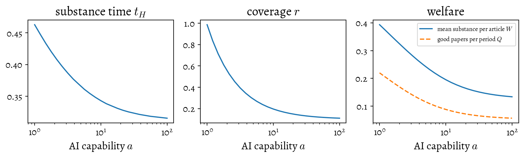
Figure 2: The free-for-all as AI drafting capability \(a\) grows: substance time per high-quality manuscript, the coverage rate \(r\), and the throughput \(Q\). \(t_H\) falls somewhat; the large damage comes from crowding.
Optimistically, we might hope that cheaper AI drafting frees up time compared to the manual alternative, allowing for more substance per paper. That does not happen under this model. The left edge of the capability sweep, \(a = 1\), is the hand-drafting equilibrium. For the high-quality tier \(H\), the substance time per manuscript \(t_H\) falls modestly as \(a\) rises, from \(0.46\) to about \(0.32\): cheaper drafting makes each manuscript cheaper, so authors choose quantity over quality. The fall is not too precipitous though: high-quality manuscripts stay above the bar (\(s_H\) drifts from \(0.68\) down to \(0.56\) scientillas, against a bar of \(0.5\) citoms), and their authors write three of them where they used to write one. For the low-quality tier \(L\), the slop authors’ output grows much faster, because a slop manuscript is nearly all drafting time: \(n_L\) rises from under \(2\) to over \(18\).
The downside is visible through the effect on the queue. The submission pool ends up \(95\%\) slop and coverage falls from roughly \(1\) to \(0.11\), so the journal publishes about four times fewer high-quality papers, even though the high-quality authors are writing more of them than before. Most of their extra manuscripts are simply never read. In the units of the model that is \(Q\) falling from \(0.22\) to \(0.06\) good papers per author-period: a journal drawing on a hundred authors goes from printing 22 good papers a period to 6. The average quality of what it does print falls too, since slop passes a full review \(12\%\) of the time and the pool is \(95\%\) slop, so most of what the journal accepts is slop.
The collapse is smooth and the equilibrium is unique. The coverage rate cancels out of every author’s problem, so there is no feedback loop to amplify anything, and no tipping point. We could expand upon that but we do not right now.
3 Policy B — Automated ban on AI-drafted manuscripts
A stylometric detector (e.g. Pangram) flags manuscripts it thinks are AI-drafted, and we desk-reject those.5 This is the only desk-reject stage; anything it passes goes into the capacity triage of the review queue. I assume the detector has true-positive rate \(\mu\), which the machine-learning literature calls its recall: it correctly flags a fraction \(\mu\) of AI-drafted manuscripts. For now, I assume it has a zero false-positive rate to keep it simple.6 Desk-rejected papers consume no reviewer time. The rest get a normal review.
Before anyone changes behaviour, notice what the detector is to an author who drafts with AI: a fee. A fraction \(\mu\) of their manuscripts is thrown away unread, so each one loses \(\mu\) times its expected return, \(\mu\,r\,b\,\Lambda_H\) for a good manuscript and \(\mu\,r\,b\,\Lambda_L\) for slop. That is a proportional levy on expected return, and since \(\Lambda_H > \Lambda_L\) it charges a good manuscript more than a slop one; a separating fee would do the opposite. We return to this with the flat congestion charge of Policy D. That by the way, is the sense in which the ban is an imperfect approximation to a fee.
Now, knowing this policy, everyone chooses how/if to write their papers. For low-quality authors, the trade-off is between the time saved by using AI and the risk of being desk-rejected. Their acceptance probability if they get past desk-rejection is the same however the manuscript was drafted, so it cancels from the comparison, and what remains is: papers per hour with AI, discounted by the survival rate \((1-\mu)\), against papers per hour by hand. They keep AI drafting while \(\mu < \mu^*(a)\), where
In this setting, the detector’s true-positive rate is pivotal, and the threshold it needs to clear depends on the time costs of producing slop. In particular, as AI capability rises toward \(f/(t_{\min}+f)\), the share of a hand-drafted slop manuscript’s time spent drafting is about \(0.91\) at my parameters. As such, a detector with a true-positive rate below that threshold deters slop authors only while AI is weak enough that \(\mu^*(a)\) is under its rate; as capability grows past that point, the same detector stops working without any change in the policy or the detector. On unmodified LLM output, the best commercial detector clears that comfortably: Pangram reports a false-negative rate of \(0.34\%\) at a false-positive rate of \(0.004\%\)(Glickenhaus et al. 2026), and independent tests put it near \(99\%\)(Russell, Karpinska, and Iyyer 2025). The rate that matters, though, is the one sustained against slop authors who rewrite to evade detection once it cuts into their earnings, and there the numbers are grim: Pangram’s own figure on AI-edited human text is \(55\)–\(65\%\)(Glickenhaus et al. 2026), and on academic abstracts a \(95\%\) rate falls to \(24\%\) once rewrite prompts are searched against the detector (Ren, Raghavan, and Garg 2026) and below \(4\%\) after a commercial humanizer (Karr et al. 2026). And because \(\mu^*(a)\) rises with capability, a ban that deters slop today can fail later without any policy change and without any decline in the detector. We ignore that twist for now.
The high-quality authors have a different behaviour threshold. Write \(V(d)\) for the best rate of expected acceptances per unit time that a high-quality author can achieve at drafting cost \(d\). High-quality authors abandon AI drafting once \((1-\mu)\,V(\delta)\) falls below \(V(f)\), that is at
\[
\mu_H(a) = 1 - \frac{V(f)}{V(\delta)}.
\]
The two thresholds are strictly ordered: \(\mu_H(a) < \mu^*(a)\) for every \(a > 1\) (at \(a = 1\) both are zero). To see this, let \(t^*_\delta\) be the substance time a high-quality author chooses when drafting with AI. A hand-drafting author could choose that same \(t^*_\delta\); it is not their optimum, so \(V(f)\) is at least what it yields, namely \(V(\delta)\,\frac{t^*_\delta + \delta}{t^*_\delta + f}\). The ratio \(\frac{t + \delta}{t + f}\) increases in \(t\), and a slop author is at \(t = t_{\min} \le t^*_\delta\), so their ratio is smaller and their threshold \(\mu^* = 1 - \frac{t_{\min} + \delta}{t_{\min} + f}\) is larger. In other words: the more substance time we invest in a manuscript, the smaller the share of its cost that AI drafting saves, so the less detection risk we will accept to keep using it. A detector therefore stops high-quality authors from using AI strictly before it stops slop authors. Neither type is ever deterred from submitting: at worst, slop authors revert to hand-drafting, which restores the hand-drafting equilibrium’s spam rate, never less. Being flagged costs a high-quality author a manuscript full of work; it costs a slop author almost nothing.
Code
mu_fix =0.5eqB = [solve_B(a, mu_fix) for a in a_grid]a_star = P["f"] / ((1- mu_fix) * (P["t_min"] + P["f"]) - P["t_min"])lo, hi =1.0, 1e4for _ inrange(60): mid = np.sqrt(lo * hi) lo, hi = (mid, hi) if mu_sub(mid) < mu_fix else (lo, mid)a_H = np.sqrt(lo * hi)fig, axes = plt.subplots(1, 3, figsize=(9.5, 3), sharex=True)grey =dict(color="#888888", alpha=0.7)axes[0].plot(a_grid, [q["tH"] for q in eqA], **grey)axes[0].plot(a_grid, [q["tH"] for q in eqB])axes[0].set_title("substance time $t_H$")axes[1].plot(a_grid, [q["r"] for q in eqA], **grey)axes[1].plot(a_grid, [q["r"] for q in eqB])axes[1].set_title("coverage $r$")axes[2].plot(a_grid, [q["thruH"] for q in eqA], **grey)axes[2].plot(a_grid, [q["thruH"] for q in eqB], label="detector ban")axes[2].plot([], [], label="free-for-all", **grey)axes[2].set_title("good papers per author-period $Q$")axes[2].legend(fontsize=8)for ax in axes: ax.set_xscale("log") ax.set_xlabel("AI capability $a$") ax.axvline(a_star, color="#555555", lw=0.8) ax.axvline(a_H, color="#555555", lw=0.8, ls="--")fig.tight_layout()plt.show()
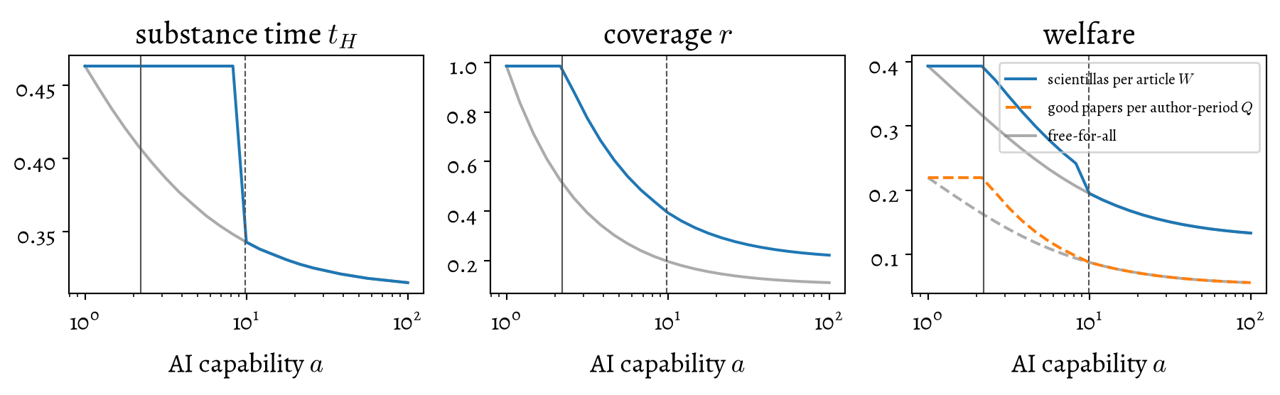
Figure 3: The detector ban at a fixed (low) true-positive rate \(\mu = 0.5\) as AI capability \(a\) grows, in the panels of Figure 2, with the free-for-all in grey for comparison. Vertical lines: where \(\mu^*(a)\) passes \(0.5\) (left) and where \(\mu_H(a)\) does (right). Left of the first line the ban deters slop authors from AI drafting, so everyone hand-drafts and the hand-drafting equilibrium of \(a = 1\) persists whatever \(a\) is; between the lines it deters only the high-quality authors, who hand-draft while slop authors keep using AI; right of the second it deters nobody and the free-for-all returns.
Three regimes appear as capability grows, with the detector’s true-positive rate held fixed. While \(\mu^*(a)\) is still below the detector’s rate (left of the solid line), even slop authors dare not use AI; everyone hand-drafts, and the hand-drafting equilibrium persists whatever \(a\) is: the ban works, at the price of forfeiting the hours that an AI would have saved. Once \(\mu^*(a)\) climbs past the detector (between the lines), the ban’s only behavioural effect is on the wrong people. High-quality authors still find AI not worth the risk and hand-draft, writing one manuscript where they could have drafted three; slop authors draft with AI, submit at full rate, and write off the fraction \(\mu\) that is desk-rejected as a cost of doing business. The ban thins the queue here because \((1-\mu)\) chokes the inflow of spam, rather than because anyone has stopped spamming; the good authors’ fewer, fuller papers raise the average quality of what is printed, not the count. Once \(\mu_H(a)\) climbs past the detector too (right of the dashed line), the ban deters nobody. Both author types draft with AI, the detector desk-rejects the same fraction \(\mu\) of each type’s manuscripts, and so long as the queue is congested, the review slots freed by desk rejection compensate for the good manuscripts lost, so the free-for-all equilibrium returns unchanged. Read against the detector instead, at fixed capability, the same three regimes run in reverse: nothing below \(\mu_H\), a tax on the compliant between \(\mu_H\) and \(\mu^*\), and the hand-drafting equilibrium above \(\mu^*\). If we instead hold capability \(a\) fixed but raise the true-positive rate \(\mu\), the same three regimes appear in the opposite order: below \(\mu_H\) the ban changes nothing; between \(\mu_H\) and \(\mu^*\) it taxes only the compliant; above \(\mu^*\) the hand-drafting equilibrium returns.
The standard objection to a ban is that it takes the time savings of AI drafting away from the compliant. My model agrees that the ban forfeits those savings, but so does the free-for-all, which converts them into extra manuscripts that mostly go unread. The savings are only worth having under a policy that can turn them into published papers, and that is what the submission fee of Policy C does.
4 Policy C — submission fees
Under this policy, we charge \(P\) per submission, allow anything, and triage and review whoever pays for it. To be clear: this is not on the table for the Alignment Journal, but is included as a baseline.
As you read this section you will note that we are talking about princely submission fees, relative to the academic norm. This is because of the bonkers economy of academic publishing which pours vast amounts of labour into producing papers, much of which is effectively un-budgeted.
I could estimate the “value” of the paper in a few ways — the effective of a paper in getting tenure, the amount of submission fee that an author seems prepared pay, or the approximate value the papers have as represented by the dollar cost of the hours that go into a typical one.
I chose the last here, since it seems the easiest to estimate (I’ve written papers), but in some ways this leads to surprisingly large valuations: it shows that papers are extremely expensive in time cost, even though academics tend to have smaller cash budgets to pay in submission fees than this time cost would indicate.
Whether anyone would be prepared to pay fees obviously depends on not just their time cost, which is sunk, but the “value” of the venue (conference, journal) to which they submit, which is also nebulous. For reference, submitting to and attending a top tier conference can cost ~USD5000 in travel, registration, and accommodation fees.
An economist would say that submission fees are always charged, in waiting time if not in cash, and a journal chooses a mix of the two whether or not it admits to pricing (Cotton 2013). This doesn’t change how it feels to be charged such a fee, nor the fact that many authors have no cash budget to pay it. Nonetheless…
Recall that a submission’s expected private return is \(b\) times its acceptance probability: \(r\,b\,\Lambda_L\) for slop, and roughly \(r\,b\,\Lambda_H\) — much larger — for a high-quality paper. Any fee between those two numbers is separating: submitting slop now loses money, while submitting good work still pays. Nobody is forced back to hand-drafting, because the fee remains the same however the paper was drafted — which is fine, since here at least we don’t care about provenance except as a proxy for spamminess.
If the submission fee is too low, slop authors keep entering until congestion drives their expected return down to the fee, \(r\,b\,\Lambda_L = P\). That pins the coverage rate at \(r = P/(b\,\Lambda_L)\): slop manuscripts fill every review slot that high-quality manuscripts do not. Raising \(P\) buys back coverage, but the accepted papers stay mostly slop until the fee exceeds the value a slop author places on each submission.
Full exclusion of slop is sadly expensive. A slop author facing an uncongested queue (\(r = 1\)) expects \(b\,\Lambda_L\) per submission, so the fee at which slop authors stop submitting entirely is
about an eighth of the private value of an acceptance (using my parameters). \(P^*\) does not depend on \(a\): the review depth \(h\) is fixed, so a slop manuscript’s acceptance odds remain the same however large the flood. The fee must handle all the deterring, which gives this policy the nifty feature of excluding slop authors with a single fee setting even as capabilities advance, unlike the ban, which we have to re-check as \(\mu^*(a)\) moves. At \(P^*\) every slop author stops submitting, at least if they are rational expected-value maximizers.
Code
fig, ax = plt.subplots(figsize=(6.5, 3.4))eqC = [solve_C(a) for a in a_grid]ax.plot(a_grid, [q["thruH"] for q in eqA], color="#b5541c", label="A: free-for-all")for mu, ls in ((0.6, "--"), (0.95, "-")): ax.plot(a_grid, [solve_B(a, mu)["thruH"] for a in a_grid], ls, color="#2d6e8e", label=f"B: detector, $\\mu={mu}$")ax.plot(a_grid, [q["thruH"] for q in eqC], color="#3a7d44", label="C: fee")ax.set_xscale("log")ax.set_xlabel("AI capability $a$")ax.set_ylabel("good papers per author-period $Q$")ax.legend(fontsize=8)fig.tight_layout()plt.show()
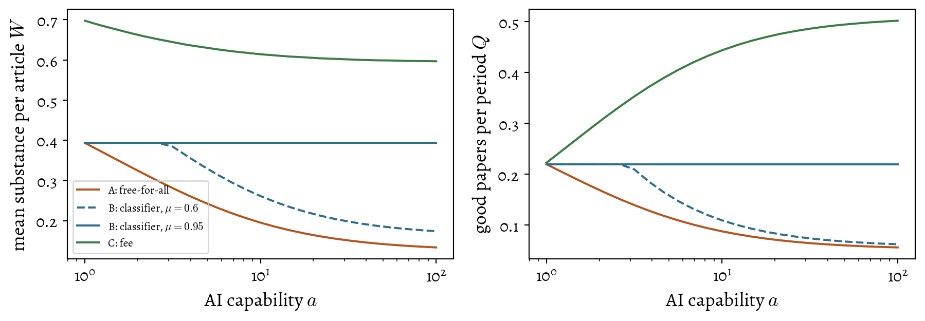
Figure 4: The three policies as AI capability grows. Detector at true-positive rate \(0.6\) and \(0.95\); fee at the full-exclusion level \(P^*\). Only the fee regime turns more capable AI into more good papers published.
Interestingly, under the fee policy, more AI capability is simply good. High-quality authors keep all the time AI saves them and spend it writing more manuscripts. Huzzah! The journal, its queue protected, has the capacity to review and publish them; and the flow of good papers into print more than doubles across the plotted range. Under the other regimes, we burn that time surplus: the ban burns it by forcing high-quality researchers back to hand-drafting, and the free-for-all converts it into unread submissions. The fee curve in the figure is computed at \(P=P^*\), the price at which slop authors stop submitting, so no slop reaches the accepted papers at all. At any lower fee, slop authors keep submitting until the queue congestion lowers their expected return to the fee, so slop manuscripts fill every review slot the high-quality manuscripts leave free, and reviewers still accept some of those.
The fee’s lead has a second component that \(Q\) does not show: the share of what gets printed that is high-quality. We can understand the gap as a mismatch between the proxy (was AI used to write this?) and the true target (was this article high-quality?). The best the ban can do, at any true-positive rate, is restore the hand-drafting equilibrium, which at these parameters means about \(58\%\) high-quality articles; a fee at \(P^*\) removes all slop from the queue, so the share is \(100\%\). An entailment of that calibration is that the journal was hypothetically going to be about \(40\%\) bullshit in the absence of AI drafting. That number follows from parameter choices I made for \(\lambda\), \(s_L\) and \(h\), which, as I said, are not crazy. Readers who believe their journal is purer than that should raise \(\lambda\) or \(h\) and watch the fee’s lead on that share shrink accordingly: the fee’s advantage arises from the hand-drafted slop it eliminates, so the dirtier we think journals already are, the stronger the case for pricing submission over policing provenance, and vice versa.
Of course, many journals cannot charge submission fees, for reasons of custom and equity, and because no matter how eloquent the justification it will still look like predatory-journal behaviour; the Alignment Journal is not exempt. The deadweight losses of dealing with spam are still imposed on someone, and in fact authors bear them, paying in lost time queuing for a review slot: with cash fees near zero, first-response delay is the de facto submission price (Azar 2005). So Policy C is useful as a benchmark: it charges for review slots in cash rather than in waiting time, which is more efficient in the raw economic sense as well as feeling better for not wasting time when we have a perfectly good substitute. The gap between it and the best policy we could feasibly adopt is the price we pay for dwelling in the earthly realm of imperfect maximizers of expected-utility and within departmental budget constraints.
A journal that did go this way would need to do some work to avoid moral hazard, or the perception of it. For example, the journal could do so by optimizing for transparency, demonstrably spending the fee revenue on reviewing.
The moral hazards look different for different types of fees. A fee charged on acceptance pays the journal for accepting, which is the predatory-journal model. A flat submission fee pays the journal either way, so the decision itself is financially neutral, but if they pay reviewers they end up ahead when rejecting. A fee refunded on acceptance charges bad papers more than good ones in expectation, but the journal keeps the cash only when it rejects, which is the opposite moral hazard.7 One fix is for forfeited fees to go to a third party, such as a disinterested charity, so that the journal has no stake in its own academic decisions. Elaborations are left as homework.
5 Policy D — authors pay to skip the detector
Authors could pay a fee \(P\) per manuscript to have it reviewed without passing through the detector. (Once again, not on the table for the Alignment Journal at the current time). Manuscripts that do not pay go through Policy B: the detector runs, and what it flags is desk-rejected. Hand-drafted manuscripts are never flagged, so their authors have no reason to pay. The fee is only ever paid by authors who drafted with AI and would rather not gamble on the detector. It imposes Policy C’s submission fee, but charges only AI drafters. Each manuscript now has three routes: draft by hand and pay nothing, draft with AI and risk desk rejection, or draft with AI and pay the fee.
Consider the slop authors first. A slop manuscript’s acceptance odds do not depend on how it was drafted, so if it reaches review it is worth \(r\,b\,\Lambda_L\) to its author however it got there. An author who drafts with AI and does not pay has a fraction \(\mu\) of their manuscripts desk-rejected, which costs them \(\mu\, r\,b\,\Lambda_L\) per manuscript in expectation. So paying the fee beats risking desk rejection only when the fee is less than \(\mu\, r\,b\,\Lambda_L\). Paying the fee beats drafting by hand only when the fee is less than \(\mu^*\, r\,b\,\Lambda_L\), by the same arithmetic that gave us \(\mu^*\) under the ban. So a slop author pays the fee only when
\[
P \;<\; \min(\mu, \mu^*)\; r\,b\,\Lambda_L.
\]
We call the right-hand side the floor fee, \(\underline{P} = \min(\mu, \mu^*)\, r\,b\,\Lambda_L\): below that price every slop author pays to skip the detector, and above it none does. Any fee the journal wants slop authors to avoid must be at least that high. At a fee above the floor, slop authors ignore the exemption option and behave as under Policy B. Below \(\mu^*\) they draft with AI and submit anyway, writing off the fraction \(\mu\) of their manuscripts that is desk-rejected as a cost of doing business. Above \(\mu^*\) they draft by hand, are never flagged, and submit at the hand-drafting equilibrium rate. The floor is lower than Policy C’s full-exclusion fee \(P^*\) by the factor \(\min(\mu, \mu^*)\,r\). Skipping the detector is worth exactly the fee it replaces, \(\mu\,r\,b\,\Lambda_L\) for slop, and in a congested queue a submission is reviewed only with probability \(r\), which scales its expected return and so the fee an author will pay (\(P^*\) was defined at \(r = 1\)). That is the floor, not the fee the journal ends up charging. The optimal exemption fee comes out above\(P^*\) at my parameters, as we see in a moment, because it is set by congestion among the high-quality authors rather than by what it takes to deter slop.
which is a fancified version of the same calculation in Policy C, differing in a few elaborations.
First, the coverage rate \(r\) no longer cancels. The fee is a fixed sum while the return scales with \(r\), so the amount an author writes now depends on how congested the queue is, and that congestion depends on how much everyone writes. The equilibrium is the point where the two agree. It is unique: a higher \(r\) makes the fee smaller relative to the return, which makes authors write more, which lengthens the queue and lowers \(r\) again. Second, they pay only while the exemption is worth buying. At a given substance choice, paying the fee beats risking desk rejection only when \(P < \mu\, r\,b\,\Lambda_H\). Call this the cap, \(\overline{P} = \mu\, r\,b\,\Lambda_H\): the detector’s fee-equivalent for a good manuscript, and therefore the highest fee the high-quality authors will pay. If the detector rarely catches anyone, nobody will pay to skip it. For those who do pay, the fee acts like an extra drafting cost. It pushes toward fewer, more substantial manuscripts, the opposite of what cheap drafting did in the first-order condition above.
Which fee? Think of the review budget as a road with a fixed number of lanes. Every submission takes a review slot, and when the queue is congested (\(r < 1\)) one more submission pushes some other manuscript out unread. If the pushed-out manuscript was good, the journal loses a good paper, and the author who did the pushing pays nothing for that loss. Economists call this a congestion externality, and the standard remedy is a congestion charge: we bill each author for the damage their submission does to everyone else’s work. In this model, the charge is easy to write down. In the congested case, the throughput is \(Q = M\,A_H/N\), where \(A_H\) is the number of accepted high-quality manuscripts per period and \(N\) is the length of the queue. One more high-quality manuscript adds \(\Lambda_H\) to \(A_H\) and one slot to \(N\), so it changes \(Q\) by \(r\,\Lambda_H - Q/N\). The author counts only the first term—the paper they might get accepted. The second term accounts for the good papers they displace, the costs of which fall on the other high-quality authors. A fee equal to the second term, converted to money at \(b\) per paper, makes the author’s calculation match the journal’s, and that is the optimal fee.
where \(\sigma_H = \lambda n_H / N\) is the high-quality share of the queue. In words: we calculate the return on a high-quality submission, discounted by the share of the queue that is high-quality. We must also set the fee above the floor \(\underline{P}\), so that slop authors don’t pay it, and yet below the cap \(\overline{P}\), so that high-quality authors do. That gives
\[
P_D \;=\; \min\!\Big\{\max\{P^\circ,\; \underline{P}\},\; \overline{P}\Big\}.
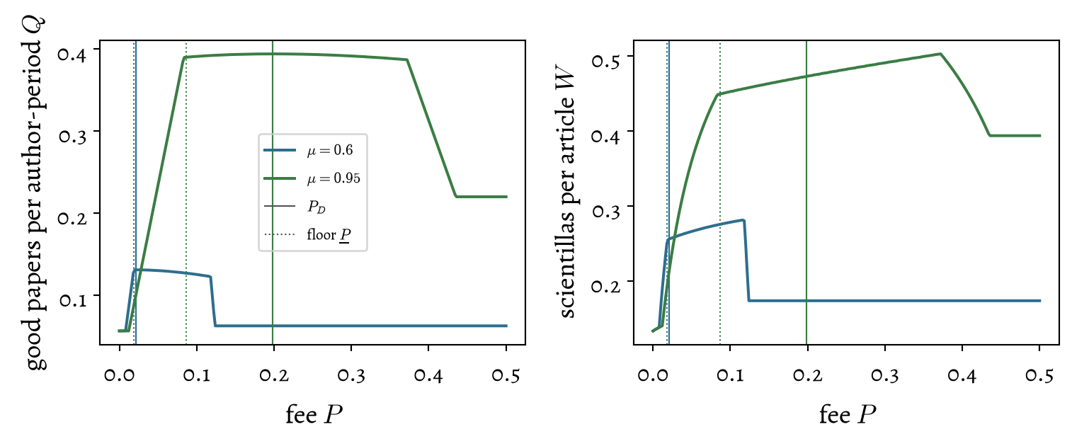
\] Everything on the right depends on the equilibrium, and the equilibrium depends on the fee, so we solve this by numerically iterating to convergence. Is the formula right? Figure 5 checks it the slow way: we hold \(a\) and \(\mu\) fixed, try every fee \(P\) from zero upward, solve for the equilibrium at each, and plot the resulting throughput \(Q\). The fee at which that curve peaks is the best fee the journal could charge, found by search rather than by formula; the solid vertical line marks the formula’s predicted best fee, and they agree. The folded cell after the figure repeats that comparison at four capability levels, from \(2\) to \(100\), and six true-positive rates, from \(0.24\) to \(0.993\), and reports the largest amount by which charging the formula fee falls short of the best fee found by search. It is zero at every point of the grid. When the congestion charge \(P^\circ\) is below the cap, the best fee is \(P^\circ\) itself. When \(P^\circ\) would exceed the cap, the best the journal can do is charge the cap: any higher and the high-quality authors stop paying, take their chances with the detector, and \(Q\) falls off the cliff visible in Figure 5. At my parameters, the congestion charge is always above the floor, so the floor never matters. When the queue is uncongested, nobody displaces anybody, the charge is zero, and \(P_D\) drops to the floor, which at \(\mu = 1\) is \(\mu^*\,b\,\Lambda_L\), a fraction \(\mu^*\) of the \(P^*\) of Policy C, because a slop author who cannot slip past the detector still has hand-drafting to fall back on.
Code
def respond_D(r, a, mu, fee, p=P):"""Best responses at coverage r when a fee buys exemption from the detector. Each manuscript takes one of three routes: hand-draft free, AI-draft and risk the desk, or AI-draft and pay. Returns queue load and accepted count per type.""" delta = p["f"] / a ret = r * p["b"] * accept_H(T_GRID, p) routes = [(ret / (T_GRID + p["f"]), p["f"], 1.0, "hand"), ((1- mu) * ret / (T_GRID + delta), delta, 1- mu, "risk"), ((ret - fee) / (T_GRID + delta), delta, 1.0, "pay")] obj, dH, wH, H_mode =max(routes, key=lambda o: o[0].max()) tH = T_GRID[int(np.argmax(obj))] loadH = p["lam"] * p["T"] / (tH + dH) * wH piL = r * p["b"] * accept_L(p) routes = [(piL / (p["t_min"] + p["f"]), p["f"], 1.0, "hand"), ((1- mu) * piL / (p["t_min"] + delta), delta, 1- mu, "risk"), ((piL - fee) / (p["t_min"] + delta), delta, 1.0, "pay")] _, dL, wL, L_mode =max(routes, key=lambda o: o[0]) loadL = (1- p["lam"]) * p["T"] / (p["t_min"] + dL) * wLreturndict(loadH=loadH, loadL=loadL, aH=loadH * accept_H(tH, p), aL=loadL * accept_L(p), tH=tH, H_mode=H_mode, L_mode=L_mode)def solve_D(a, mu, fee, p=P, iters=60):"""Exemption fee: coverage no longer cancels from anyone's problem, so bisect for the fixed point in r. At a jump in either type's response that type mixes, so blend the two sides of the jump in the proportion that fills the queue.""" M = p["R"] / p["h"] lo, hi =1e-6, 1.0for _ inrange(iters): mid =0.5* (lo + hi) q = respond_D(mid, a, mu, fee, p)ifmin(1.0, M / (q["loadH"] + q["loadL"])) > mid: lo = midelse: hi = mid r =0.5* (lo + hi) qlo, qhi = respond_D(lo, a, mu, fee, p), respond_D(hi, a, mu, fee, p) Nlo, Nhi = qlo["loadH"] + qlo["loadL"], qhi["loadH"] + qhi["loadL"] congested = r <1-1e-6 alpha = np.clip((M / r - Nhi) / (Nlo - Nhi), 0, 1) if congested andabs(Nlo - Nhi) >1e-9else1.0 mix =lambda k: alpha * qlo[k] + (1- alpha) * qhi[k] aH, aL, N = mix("aH"), mix("aL"), mix("loadH") + mix("loadL") sH = p["theta"] * (alpha * qlo["aH"] * np.sqrt(qlo["tH"])+ (1- alpha) * qhi["aH"] * np.sqrt(qhi["tH"])) / aH W = aH * sH / (aH + aL) if aH + aL >0else0.0returndict(r=r, W=W, thruH=r * aH, tH=mix("tH"), sH=sH, N=N, H_pays=qlo["H_mode"] =="pay", floor=min(mu, mu_star(a, p)) * r * p["b"] * accept_L(p), charge=p["b"] * r * aH / N if congested else0.0)def fee_D(a, mu, p=P, eps=1e-3, iters=200):"""Q-optimal fee: the fixed point of P = max(b Q / N, floor + eps), capped at the largest fee the high-quality authors will pay rather than risk the desk.""" fee = p["b"] * accept_L(p)for _ inrange(iters): q = solve_D(a, mu, fee, p) new =max(q["charge"], q["floor"] + eps)ifabs(new - fee) <1e-7:break fee =0.5* (fee + new)ifnot solve_D(a, mu, fee, p)["H_pays"]: lo, hi =0.0, feefor _ inrange(40): mid =0.5* (lo + hi) lo, hi = (mid, hi) if solve_D(a, mu, mid, p)["H_pays"] else (lo, mid) fee = loreturn fee
Code
from matplotlib.lines import Line2Dfees = np.linspace(0.0, 0.5, 251)fig, axq = plt.subplots(figsize=(6.5, 3.2))for mu, col in ((0.6, "#2d6e8e"), (0.95, "#3a7d44")): sweep = [solve_D(100, mu, f) for f in fees] axq.plot(fees, [q["thruH"] for q in sweep], color=col, label=f"$\\mu = {mu}$") fd = fee_D(100, mu) axq.axvline(fd, color=col, lw=0.8) axq.axvline(solve_D(100, mu, fd)["floor"], color=col, ls=":", lw=0.8)axq.set_ylabel("good papers per author-period $Q$")axq.set_xlabel("fee $P$")handles, labels = axq.get_legend_handles_labels()handles += [Line2D([], [], color="#555555", lw=0.8), Line2D([], [], color="#555555", ls=":", lw=0.8)]labels += ["$P_D$", r"floor $\underline{P}$"]axq.legend(handles, labels, fontsize=8)fig.tight_layout()plt.show()
Figure 5: The exemption fee at \(a = 100\): throughput \(Q\) against the fee \(P\), at two true-positive rates. Solid verticals mark the formula \(P_D\); dotted verticals mark the floor \(\underline{P}\), below which slop authors pay the fee too. The cliff on the right of each curve is where high-quality authors stop paying and take their chances with the detector.
Check the formula fee against a brute-force sweep
worst =0.0for a_chk in (2, 5, 15, 100):for mu_chk in (0.24, 0.4, 0.6, 0.8, 0.95, 0.993): best =max(solve_D(a_chk, mu_chk, f)["thruH"] for f in fees) got = solve_D(a_chk, mu_chk, fee_D(a_chk, mu_chk))["thruH"] worst =max(worst, (best - got) / best)print(f"largest throughput shortfall of the formula fee against the sweep: {100* worst:.2f}%")
largest throughput shortfall of the formula fee against the sweep: 0.00%
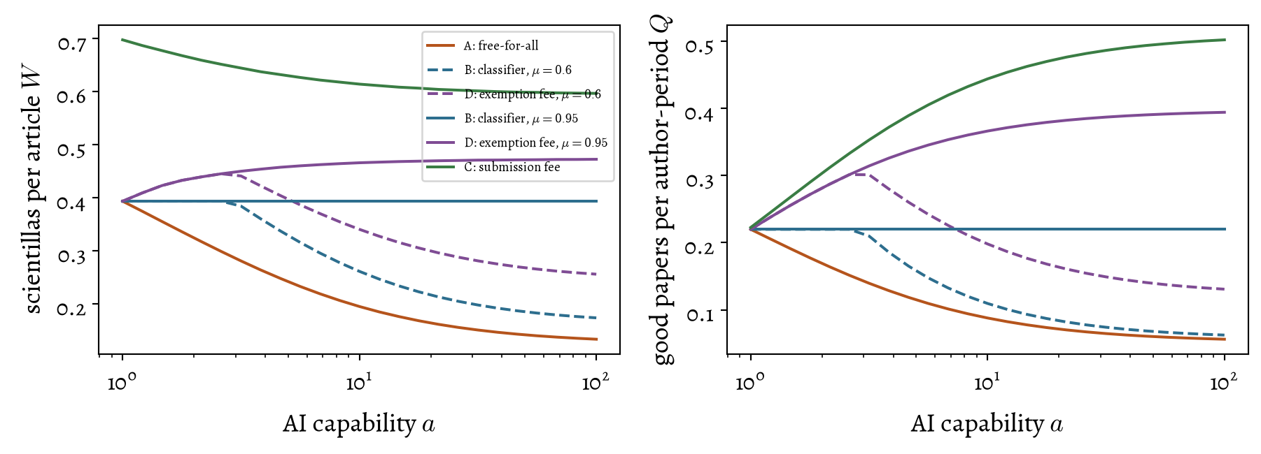
The detector’s true-positive rate does not appear in the congestion charge. In Policy D the detector does one thing: it gives AI-drafting authors a reason to pay by desk-rejecting a fraction \(\mu\) of AI-drafted, non-fee-paying manuscripts. The true-positive rate enters only the floor and the cap, both of which rise with \(\mu\) because skipping a better detector is worth more; a better detector widens the range of fees that high-quality authors will pay and slop authors will not. At a low enough true-positive rate, the cap falls below the congestion charge, and the journal can charge only what high-quality authors will still pay. Unlike \(P^*\), this fee changes as \(a\) grows, because \(Q\) and \(N\) do. This is the one place where the average-quality metric \(W\) would disagree with our overall value metric \(Q\): \(W\) is blind to volume as long as the average quality is high, so it would prefer the largest fee the high-quality authors will pay, right up to the cap. Near \(a = 1\), the fee pushes high-quality authors back to hand-drafting, because AI saves them almost nothing there, and Policy D degenerates into Policy B.
Code
fig, ax = plt.subplots(figsize=(6.5, 3.4))eqD = {mu: [solve_D(a, mu, fee_D(a, mu)) for a in a_grid] for mu in (0.6, 0.95)}ax.plot(a_grid, [q["thruH"] for q in eqA], color="#b5541c", label="A: free-for-all")for mu, ls in ((0.6, "--"), (0.95, "-")): ax.plot(a_grid, [solve_B(a, mu)["thruH"] for a in a_grid], ls, color="#2d6e8e", label=f"B: detector, $\\mu={mu}$") ax.plot(a_grid, [q["thruH"] for q in eqD[mu]], ls, color="#7f4c94", label=f"D: exemption fee, $\\mu={mu}$")ax.plot(a_grid, [q["thruH"] for q in eqC], color="#3a7d44", label="C: submission fee")ax.set_xscale("log")ax.set_xlabel("AI capability $a$")ax.set_ylabel("good papers per author-period $Q$")ax.legend(fontsize=7)fig.tight_layout()plt.show()
Figure 6: The four policies as AI capability grows. Detector and exemption fee at true-positive rate \(0.6\) and \(0.95\); submission fee at \(P^*\); exemption fee at \(P_D\). The exemption fee is between the ban and the submission fee at every capability level \(a\).
The exemption fee lands between the ban and the submission fee at every capability level in Figure 6. Above \(\mu^*\) the ban restores the hand-drafting equilibrium, \(Q \approx 0.22\) good papers per author-period at my parameters, regardless of \(a\); the exemption fee at the same true-positive rate publishes \(0.39\) at \(a = 100\) (39 a period per hundred authors, against 22), because high-quality authors keep the time AI saves them and the congestion charge stops them from spending all of it on extra manuscripts. Below \(\mu^*\), at \(\mu = 0.6\), the exemption fee roughly doubles the ban’s throughput, but both are poor, because the \(40\%\) of AI-drafted slop manuscripts that the detector misses still fill the queue. What separates the exemption fee from the submission fee is hand-drafted slop: under Policy C slop authors pay whether or not they used AI, so they stop submitting; under Policy D a slop author who drafts by hand pays nothing, is never flagged, and stays in the queue. At \(\mu = 1\) every AI drafter pays, and Policy D is Policy C levied on AI drafters alone; the slop authors who draft by hand are the whole difference.
For the Alignment Journal the exemption fee faces the same objection as the submission fee—that we would be charging money from a cash-constrained author base. Only authors who choose to pay are charged. Paying is also a disclosure: a hand-drafted manuscript is never flagged, so the only reason to buy the exemption is that the manuscript was AI-drafted. Most journals now ask authors to declare AI use but can at best partially check the claim; here it arrives with a fee attached, so it is truthful by construction. A false positive still costs a hand-drafting author their manuscript, as under the ban. And the revenue arrives in proportion to the number of AI-drafted manuscripts the journal has to review, so a journal that pays its reviewers could route it straight back into \(R\).
I am indebted to Vanessa Kosoy for helpful discussions which led to this proposal.
6 Future work
On this analysis the detector ban is a clumsy approximation to a congestion charge, and Policy D makes the charge explicit: what we are charging for is constrained review slots. Whether the Alignment Journal, or any journal, has a reasonable economic basis to adopt the ban depends on two parameters I have only guessed here:
the true-positive rate a detector can sustain against motivated rewriting, compared against a \(\mu^*\) we could estimate from the time costs of producing slop; and
how many good AI-drafted papers we would tolerate losing in the range of true-positive rates between the two thresholds.
6.1 Not modelled
Diluted review. Throughout, the journal holds review depth \(h\) fixed and rations coverage \(r\) by skipping papers, which is why every collapse above is smooth and every equilibrium unique. A journal that instead reviews everything less carefully puts congestion inside the authors’ incentives, and at some author mixes the decline becomes a fold with hysteresis: a cliff that does not reverse when capability is walked back. That variant has its own post, Diluted review; Bartolucci and Vivo (2026) works the same margin out properly in a queueing model.
Better AI prose. Everything here assumes AI lowers the cost of writing a manuscript without changing what a reviewer sees in it. Better prose breaks that in two ways. Slop presents more citoms, so \(s_L\) rises. Real but modest work reads as better than it is, an inflation I assumed away by making citoms and scientillas coincide for good authors. Polished slop and oversold real work alike look better to a reviewer with a persuasive AI polisher, without being any more useful to a reader, so the acceptance gap \(\Lambda_H - \Lambda_L\) that we need to make fees separate the classes gets narrower. As it closes, no fee separates and no detector helps, and the journal’s problem stops being desk mechanism design and becomes epistemology: telling good from bad at review, with more reviewer time per manuscript.
Better AI science. The premise that AI can write a paper but not do the science behind it is a statement about current (or really, 2024) capability. Once AI raises the substance of a manuscript as well as its polish, cheap drafting no longer buys only thinner papers: an hour of substance time buys more scientillas, and a slop author’s manuscript need not be slop. The slop-versus-quality distinction the model rests on goes with it, and so do these results.
Harmful slop. Accepted slop is harmless here; if it instead poisons training corpora (Shumailov et al. 2023) or locks in error (Qiu et al. 2025), its value is negative and everything above understates the case for keeping it out.
Many journals. There is only one journal here; with many, slop authors send their manuscripts to whichever is least strict and there is a race to the bottom, which is a different and worse game.
False positives. The detector is assumed never to flag a hand-drafted manuscript, which is unlikely in practice; a false positive costs a compliant author a manuscript full of work, so even a small rate changes the outcomes near \(\mu_H\) and, worse, erodes trust.
Reputations. If publishing slop were reputationally harmful, the return to slop would change and the amount of spam might also be moderated.
7 Ballpark real-world estimates
The model prices everything in units of \(b\), the value of one accepted paper to its author, so a fee in dollars needs a guess at \(b\) in dollars. My best anchor is cost: a typical ICLR paper has historically taken about four researcher-months, and a careerist keeps spending that only if an acceptance is worth at least as much to them, so four researcher-months is a lower bound on \(b\). At USD 5,000 to USD 15,000 per researcher-month, from a PhD stipend to a fully loaded academic salary, that puts \(b\) at USD 20,000 to USD 60,000. I will carry both ends through.
Under Policy C the fee at which slop authors stop submitting is \(P^* = b\,\Lambda_L\), which at my parameters is about an eighth of \(b\): USD 2,500 to USD 7,500 per submission.
Under Policy D with a Pangram-grade detector, taking the true-positive rate from credible independent tests (Russell, Karpinska, and Iyyer 2025) as \(\mu = 0.993\) (i.e. \(99.3\%\)) with no false positives, that rate clears the large-\(a\) limit, i.e. \(\mu^*(a) \le 0.91 < \mu\) for every \(a\), so slop authors draft by hand, take their chances and never pay the fee. The fee is then a pure congestion charge. It rises slowly with \(a\), from \(0.16\,b\) at \(a = 2\) to \(0.20\,b\) at \(a = 100\). Call it a fifth of \(b\): USD 4,000 to USD 12,000 per AI-drafted submission. The floor is \(0.05\)–\(0.09\,b\), well below that, so slop authors do not pay at any fee in this range. Those dollar figures assume the detector wins the arms race. At the \(24\%\) that survives a rewrite attack, the exemption fee collapses to \(0.007\,b\), a few hundred dollars, because skipping a detector that catches a quarter of manuscripts is worth little to anyone, and throughput barely improves on the free-for-all (\(0.07\) against \(0.06\) good papers per author-period). A detector that slop authors can defeat prices nothing.
The ban has a price too, paid in time rather than money. Above \(\mu^*\) every high-quality author drafts by hand, so each of their manuscripts costs \(f - \delta\) more time than it would with AI, about \(0.5\) time units at \(a = 100\). On the same anchor, a paper takes about \(0.96\) time units and four researcher-months, so the ban costs a good author about two researcher-months per manuscript: roughly half of \(b\), or USD 10,000 to USD 30,000. That is between two and three times the exemption fee, and the journal does not even collect it. A second way to price the ban gives its fee-equivalent directly: the exemption fee at which a high-quality author would be as well off as under the ban is \(0.44\,b\) at \(a = 100\), USD 9,000 to USD 26,000, falling to \(0.19\,b\) at \(a = 2\), USD 4,000 to USD 11,000, where AI saves little drafting time and the ban costs little. Either way the ban is a fee of the same order as the exemption fee, levied in time, on the good authors only, and collected by nobody.
The ideal exemption fee face value is higher than the submission fee. Under Policy C the fee only has to keep slop authors out, and once they are gone the queue is uncongested, so there is no congestion to charge for. Under Policy D the slop authors who draft by hand stay, the queue stays congested, and the fee is a congestion charge on the high-quality authors.
Both fees are large next to what journals that do charge actually ask; economics journals charge around USD 100–300 per submission, I believe. Either the going rate is low, or \(b\) is smaller than I have guessed for most authors, or my \(\Lambda_L\) is too high. A journal whose full review lets through fewer than \(12\%\) of slop manuscripts needs a proportionately smaller fee, since \(P^*\) scales with \(\Lambda_L\).
The detector reads style, not substance, and the two are coming apart: in the neighbouring market for cover letters, an AI writing tool cut the correlation between text quality and callbacks by half (Cui, Dias, and Ye 2025).↩︎
Jess Riedel points out that the refundable fee which just excludes slop, \(b\,\Lambda_L/(1-\Lambda_L)\), induces the same substance time and throughput as the flat fee \(P^*\), while a good author pays only about a quarter as much in expectation. They must front slightly more cash, though, so it does not help authors who have none.↩︎