Advice to pivot into AI Safety is likely miscalibrated

1.1 Modeling the Sabbatical gamble

1.2 Decision Threshold

With these inputs, we can calculate the total expected value (EV) of her sabbatical gamble. The full derivation is in Appendix A, but here’s the result:

\[ \boxed{ \Delta \mathrm{EV}\_\rho(p) =\frac{1-e^{-(r p+\rho)\ell}}{r p+\rho}\left(\frac{\Delta u r p}{\rho}-c\right). } \]

This formula looks complex, but the logic is simple. The whole decision hinges on the sign of the term in brackets: \[ \left(\frac{\Delta u r p}{\rho}-c\right) \] This directly compares the expected gain rate (the upside \(\Delta u\) multiplied by the success rate \(rp\) and adjusted for discounting \(1/\rho\)) with the burn rate (\(c\)). That prefactor scales this value according to the length of Alice’s runway and her discount rate.

The EV is positive if and only if the gain rate exceeds the burn rate. This means Alice’s decision boils down to a simple question: is her per-application success probability, \(p\), high enough to make the gamble worthwhile?

We can find the exact break-even probability, \(p^*\), by setting the gain rate equal to the burn rate. This gives a much simpler formula for Alice’s decision threshold:

\[ \boxed{\,p^*=\frac{c\,\rho}{r\,\Delta u}\,}. \]

If Alice believes her actual \(p\) is greater than this \(p^*\), the pivot has a positive expected value. If \(p < p^*\), she should not take the sabbatical, at least on these terms.

1.3 What This Model Tells Alice

This simple threshold \(p^*\) gives us a clear way to think about her decision:

1. The bar gets higher: The threshold \(p^*\) increases with higher costs (\(c\)), shorter timelines, or greater impatience (\(\rho\)). If her sabbatical is expensive or she’s in a hurry, she needs to be more confident of success.

2. The bar gets lower: The threshold \(p^*\) decreases with more opportunities (\(r\)) or a higher upside (\(\Delta u\)). If the job offers a massive impact gain or she can apply to many roles, she can tolerate a lower chance of success on any single one.

3. Runway doesn’t change the threshold: Notice that the runway length \(\ell\) isn’t in the \(p^*\) formula. A longer runway gives her more expected value (or loss) if she does take the gamble, but it doesn’t change the break-even probability itself.

4. The results are fragile to uncertainty: This model is highly sensitive to her estimates. If she overestimates her potential impact (a high \(\Delta u\)) or underestimates her time preference (a low \(\rho\)), she’ll calculate a \(p^*\) that is artificially low, making the pivot look much safer than it is.¹

5. The key unknown: Even with a perfectly calculated \(p^*\), Alice still faces the hardest part: estimating her own actual success probability, \(p\).

That \(p\) is, essentially, her chance of getting an offer. It depends not only on the number of jobs available but crucially on the number and quality of the other applicants.

All that said, this is a relatively “optimistic” model. If Alice attaches a high value to getting her hands dirty in AI safety work, she might be willing to accept a remarkably low \(p\). We’ll see that in the worked example. Hold that thought, though, because I’ll argue that this personal decision rule can be pretty bad at maximizing total impact.

1.4 Worked example

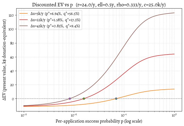
Let’s plug in some plausible numbers for Alice. She’s a successful software engineer who earns \(w_0=180\)k$/year, donates \(d_0=18\)k$/year after tax, and has no on-the-job impact \(\mathcal{I}_0=0\) (i.e. no net harm and no net good). That means Alice earns \(w_0=180\) and donates \(d_0=18\). A target role offers \(w_1=120\), \(d_1=0\), and \(\mathcal{I}_1=100\). Set \(\alpha=1\), a runway of \(\ell=0.5\) years, an application rate of \(r=24\)/year, a discount of \(\rho=1/3\), and a burn of \(c=50\). Then \(\Delta u = (120+0+100)-(180+18+0)=22\) and \[ p^*=\frac{c\rho}{r\Delta u} = \frac{50\cdot\frac{1}{3}}{24\cdot 22} \approx \boxed{3.16\%}. \] Over six months, the chance of at least one success at \(p^*\) is \(q^*=1-e^{-rp^*\ell}\approx \boxed{31.5\%}\). Alice’s expected sabbatical length is \(\mathbb{E}[\tau]=\frac{1-e^{-rp^*\ell}}{rp^*}\approx \mathbf{0.416}\ \text{years (≈5.0 months)}\); conditional on success, it’s \(\mathbb{E}[\tau\mid \text{success}]\approx \mathbf{0.234}\ \text{years (≈2.8 months)}\). Under these assumptions, we expect the sabbatical to break even: the job offers enough upside to compensate for a higher-than-even risk of failure.

We plot a few values to help Alice visualize the trade-offs for different upsides \(\Delta u\).

To play around with the assumptions, try our interactive Pivot EV Calculator (source: danmackinlay/career_pivot_calculator).

2.1 From personal gambles to field strategy

Our goal is to move beyond Alice’s private break-even (\(p^*\)) and calculate the field’s welfare-maximizing applicant pool size (\(K^*\)). \(K^*\) is how many “Alices” the field can afford to have rolling the dice before the costs of failures outweigh the value of successes.

To analyze this, we must shift our model in three ways:

1. Switch to a Public Ledger: From a field-level perspective, private wages and consumption are transfers and drop out of the analysis. What matters is the net production of public goods (i.e., impact).

2. Distinguish Public vs. Private Costs: The costs are now different.

   • Private Cost (Part A): \(c\) included Alice’s full opportunity cost (foregone wages, etc.).
   • Public Cost (Part B): We now use \(\gamma\), which captures only the foregone public goods during a sabbatical (e.g., \(\gamma = \mathcal {I}_0 + d_0 + \varepsilon\): baseline impact, baseline donations and externalities).

3. Move from Dynamic Search to Static Contest: Instead of an individual’s dynamic search, we’ll use a static “snapshot” model of the entire field for one year. We assume there are \(N\) open roles and \(K\) total applicants that year.

2.2 The Field-Level Model: Assumptions

Here’s the minimally complicated version of our new model:

• There are \(K\) total applicants and \(N\) open roles per year.
• Each applicant \(k\) has a true, fixed potential impact \(J^{(k)}\) drawn i.i.d. from the talent distribution \(F\).
• Employers perfectly observe \(J^{(k)}\) and hire the \(N\) best candidates. (This is a strong, optimistic assumption about hiring efficiency).
• Applicants do not know their own \(J^{(k)}\), only the distribution \(F\).

The intuition is that the field benefits from a larger pool \(K\) because it increases the chance of finding high-impact candidates. But the field also pays a price for every failed applicant.

2.3 Benefits vs. Costs on the Public Ledger

Let’s define the two sides of the field’s welfare equation.

The Marginal Benefit (MV) of a Larger Pool

A larger pool \(K\) helps us find better candidates. We care about the marginal value of adding one more applicant to the pool, which we define as \(\mathrm{MV}_K\). This is the expected annual increase in impact from widening the pool from \(K\) to \(K+1\). (Formally, \(\mathrm{MV}_K := \mathbb{E}[S_{N,K+1}] - \mathbb{E}[S_{N,K}]\), where \(S_{N,K}\) is the total impact of the top \(N\) hires from a pool of \(K\)).

The Marginal Cost (MC) of a Larger Pool

The cost is simpler. When \(K > N\), adding one more applicant results (on average) in one more failed pivot. This failed pivot costs the field the foregone public good during the sabbatical. We define the social burn rate per year as \(\gamma\). To compare this to the annual benefit \(\mathrm{MV}_K\), we need the total present value of this foregone impact. We call this \(L_{\text{fail},\delta}\) (the PV of one failed attempt). (This cost is derived in Appendix B as \(L_{\text{fail},\delta}=\gamma\,\frac{1-e^{-\delta\ell}}{\delta}\)).

We do not model employer congestion from reviewing lots of applicants — the rationale is that it’s empirically small because employers stop looking at candidates when they’re overwhelmed (J. Horton and Vasserman 2021).²

2.4 Field-Level trade-offs

We can now find the optimal pool size \(K^*\). The total public welfare \(W (K)\) peaks when the marginal benefit of one more applicant equals the marginal cost.

As derived in Appendix B, the total welfare \(W(K)\) is maximized when the present value of the annual benefit stream from the marginal applicant (\(\mathrm{MV}_K / \delta\)) equals the total present value of their failure cost (\(L_{\text{fail},\delta}\)). \[ \frac{\mathrm{MV}_K}{\delta} = L_{\text{fail},\delta} \] Substituting the expression for \(L_{\text{fail},\delta}\) and cancelling the discount rate \(\delta\) yields a very clean threshold: \[ \boxed{\,\mathrm{MV}_K = \gamma\,(1-e^{-\delta\ell})\,}. \] This equation underlies the field-level problem. The optimal pool size \(K^*\) is the point where the expected annual marginal benefit (\(\mathrm{MV}_K\)) falls to the level of the total foregone public good from a single failed sabbatical attempt.

2.5 The Importance of Tail Distributions

How quickly does \(\mathrm{MV}_K\) shrink? Extreme value theory tells us it depends entirely on the tail of the candidate-quality distribution, \(F\). The shape of the tail determines how quickly returns from widening the applicant pool diminish.

We consider two families (the specific formulas are in Appendix B):

• Light tails (e.g., Exponential): In this world, candidates vary, but the best isn’t transformatively better than average. Returns diminish quickly: the marginal value \(\mathrm{MV}_K\) shrinks hyperbolically (roughly as \(1/K\)).

• Heavy tails (e.g., Fréchet): This captures the “unicorn” intuition. Returns diminish much more slowly. If the tail is heavy enough, \(\mathrm {MV}_K\) decays extremely slowly, justifying a very wide search.

2.6 Implications for Optimal Pool Size

This difference in diminishing returns greatly affects the optimal pool size \(K^*\). The full solutions for \(K^*\) are in Appendix B.

With light tails, there’s a finite pool size beyond which ramping up the hype (increasing \(K\)) reduces net welfare. Every extra applicant burns \(L_{\text{fail},\delta}\) in foregone public impact while adding an \(\mathrm{MV}_K\) that shrinks rapidly.

With heavy tails, it’s different. As the tail gets heavier, \(K^*\) explodes. In very heavy-tailed worlds, very wide funnels can still be net positive. We may decide it’s worth, as a society, spending a lot of resources to find the few unicorns.

We set the expected impact per hire per year to \(\mu_{\text{imp}}=100\) (impact dollars/yr) to match Alice’s hypothetical target role. This is just for exposition.

We can, of course, plot this.

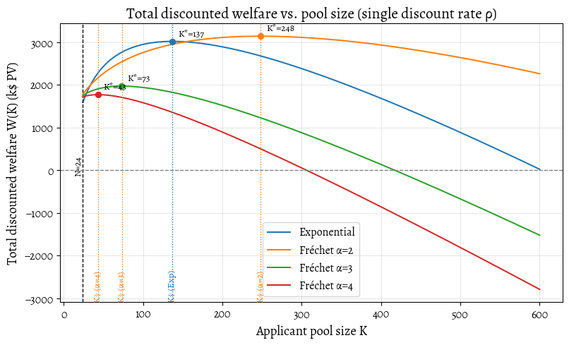
δ=0.333/yr, L_fail=8.29 impact-$ (PV)
Exponential: K*=800 (boundary), W*=25869.7
Fréchet α=1.8: K*=800 (boundary), W*=50300.4
Fréchet α=2.0: K*=800 (boundary), W*=40229.2
Fréchet α=3.0: K*=800 (boundary), W*=19116.8

• This plot shows total net welfare \(W (K)\) and marks the maximum \(K^*\) for each family, so we can see where welfare peaks. The dashed line at \(K=N\) shows when failures begin: \((K>N\Rightarrow K-N\) people each impose a public cost of \(L_{\text{fail},\delta})\). The markers show \(K^*=\arg\max W(K)\) — the pool size beyond which widening would reduce total impact.
• Units: \(B(K)\) is in impact dollars per year and is converted to PV by multiplying by \(H_\delta=\frac{1}{\delta}\). The subtraction uses the discounted per-failure cost \(L_{\text{fail},\delta}=\gamma\,\frac{1-e^{-\delta\ell}}{\delta}\).
• Fréchet curves use the large-\(K\) asymptotic \(B(K)\approx s\,K^{1/\alpha}C_N\) (with \(s=\mu_{\text{imp}}/\Gamma(1-1/\alpha)\)). We could compute the exact \(B(K)\) for Fréchet, but the asymptotic is good enough to illustrate the qualitative behaviour.
• We treat future uncertainties about role duration, turnover, or project lifespan as already captured by the overall discount rate \(\delta\).

We can combine these perspectives to visualize the tension between private incentives and public welfare.

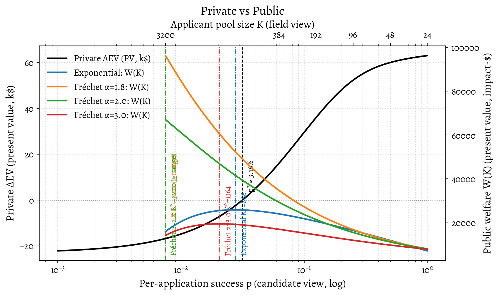
p* (private) = 3.16%
Exponential: K*=868, p(K*)≈2.76%
Fréchet α=1.8: K*=3200 (boundary), p(K*)≈0.75%
Fréchet α=2.0: K*=3200 (boundary), p(K*)≈0.75%
Fréchet α=3.0: K*=1164, p(K*)≈2.06%

We combine the private and public views using an illustrative mapping from pool size to success probability: \(p\approx \beta N/K\), where \(\beta\) bundles screening efficiency, and in this figure \(\beta=1\). The black curve (left axis) shows a candidate’s private expected value (EV) as a function of success probability \(p\). The coloured curves (right axis) show the field’s welfare, \(W(K)\). The private break-even point \(p^*\) (black dashed line) can fall far to the left of the field-optimal point \(p(K^*)\) (coloured vertical lines). This gap marks the region where individuals, acting rationally, are incentivized to enter even though, from the candidate’s perspective, the field is already saturated or oversaturated.

3.1 The Counterfactual Impact Model

In Part A, Alice’s upside \(\Delta u\) included the absolute impact \(\mathcal{I}_1\). But her true impact is counterfactual: it’s the value she adds compared to the next-best person who would have been hired if she hadn’t applied.

How can she estimate this? She doesn’t know her own quality (\(J^{(k)}\)) relative to the pool. If we assume she is, from the field’s perspective, just one more “draw” from the talent distribution \(F\) (formally: applicants are exchangeable), then her expected counterfactual impact from the decision to apply is exactly the marginal value of adding one more applicant: \(\mathrm{MV}_K\) (from Part B).

This \(\mathrm{MV}_K\) is her ex-ante expected impact before the gamble is resolved. But her EV calculation (from Part A) needs the upside conditional on success.

Let \(\mathcal{I}_{CF}\) be this value: the expected counterfactual impact given she succeeds and gets the job. Let \(q_K\) be her overall probability of success in a pool of size \(K\). (In the static model of Part B, if she joins a pool of \(K\) others, there are \(K+1\) applicants for \(N\) slots, so \(q_K \approx N/(K+1)\)). If her attempt fails (with probability \(1-q_K\)), her counterfactual impact is zero.

Therefore, the ex-ante expected impact \(\mathrm{MV}_K\) is simply the probability of success multiplied by the value of that success:

\[ \mathrm{MV}_K = (q_K \cdot \mathcal{I}_{CF}) + ((1-q_K) \cdot 0) = q_K \cdot \mathcal{I}_{CF}. \]

This gives us the key value Alice needs. Her expected counterfactual impact, conditional on success is:

\[ \boxed{\mathcal{I}_{CF} = \frac{\mathrm{MV}_K}{q_K}.} \]

Alice can now recalibrate her private decision from Part A. She defines a counterfactual private surplus, \(\Delta u_{CF}\), by replacing the naive absolute impact \(\mathcal{I}_1\) with her sophisticated counterfactual estimate \(\mathcal{I}_{CF}\).

This changes the dynamics entirely. In Part A, the value of the upside (\(\Delta u\)) was fixed. Now, the value of the upside (\(\Delta u_{CF}\)) itself depends on the pool size \(K\).

As \(K\) grows, both \(\mathrm{MV}_K\) (the marginal value) and \(q_K\) (the success chance) decrease. How \(\mathcal{I}_{CF}\) behaves depends on which decreases faster—the marginal value or the success chance—a property determined by the tail of the impact distribution \(F\).

3.2 The Dynamics of Counterfactual Impact

The behaviour of \(\mathcal{I}_{CF}\) leads to radically different incentives depending on the tail shape of the talent pool.

3.3 Alice Revisited

Alice revisited. With light‑tailed assumptions, \(\mathcal{I}_{CF}\) equals the population mean \(\mu\) and is too small to offset Alice’s pay cut and lost donations — her counterfactual surplus is negative regardless of \(K\). Under heavy‑tailed assumptions, \(\mathcal{I}_{CF}\) rises with \(K\); across a broad range of conditions, the pivot can become attractive despite large pay cuts (i.e. if Alice could truly be a unicorn). The sign and size of this effect hinge on the tail parameter and scale, which we haven’t measured yet.

3.4 Visualizing Private Incentives vs. Public Welfare

We can now visualize the dynamics of private, public, and counterfactual private valuations by assuming an illustrative mapping between pool size and success probability: \(p\approx \beta N/K\). This lets us see how incentives change as the field gets more crowded (moving left on the x-axis).

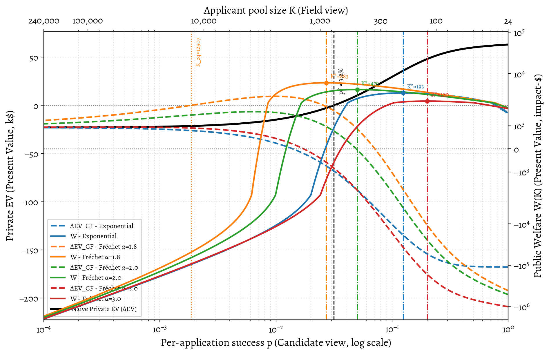
3.5 Visualizing the Misalignment

This visualization brings all three models together, using Alice’s parameters to illustrate the tensions between private incentives and public good. The plot is dense, but it we can read threee key dynamics off it:

1. The Information Gap (A vs. C): The “Naive EV” (A, black solid line) is far more optimistic than the “Counterfactual EV” (C, dashed colored lines). An applicant using the simple model from Part A—ignoring their displacement effect—will drastically overestimate the personal EV of pivoting.
2. The Impact of Costs (C): In light-tailed worlds (Exponential, purple; Fréchet \(\alpha=3.0\), red), the counterfactual impact is modest. For an applicant like Alice, with her high opportunity costs (a \(\approx 50k\) annual burn rate plus \(18k\) in foregone donations), once there are more applicants than jobs, her impact isn’t large enough to offset her personal financial losses. Her sophisticated EV (dashed line) is therefore negative across the plotted range, implying she should not attempt the pivot in this scenario.
3. The Structural Misalignment (B vs. C): This is the core problem. In the heavy-tailed “unicorn” worlds where pivoting is privately rational (green, orange), the socially optimal pool size (\(K^*\), the peak of the solid welfare lines) is far smaller than the private equilibrium (\(K_{eq}\), where the dashed EV lines cross zero). The system incentivizes massive over entry in the field’s own terms.

3.6 Why Does This Happen?

The trite answer is: there are no feedback mechanisms so we should expect alignment to be accidental and transitory when it occurs. A deeper answer is that we might imagine putting in feedback mechanisms but then we will need to decide what to align to. There is a conflict between the private cost of trying and the social cost of failing.

We can find the two different “stop” signals that define the optimum vs. the equilibrium:

1. The Social Optimum (\(K^*\)): The field’s total welfare (Part B) peaks when the marginal impact of one more applicant (\(\mathrm {MV}_K\)) drops to equal the social cost of their (likely) failed attempt. For Alice, this cost is the public good she stops producing during her sabbatical—primarily her donations.
   • Social Cost of Failure (\(\gamma\)): \(\mathbf{\$18k}\)/year.
2. The Private Equilibrium (\(K_{eq}\)): A sophisticated Alice (Part C) stops applying when her private EV becomes zero. This happens when the marginal impact she can expect to have (\(\mathrm {MV}_K\), which she shares with other applicants) drops to equal her effective private cost hurdle per application. As derived in Appendix C, this hurdle is \(\frac{c\rho}{r}\).
   • Private Cost Hurdle (\(\frac{c\rho}{r}\)): \(\frac{50k \cdot 1/3}{24} \approx \mathbf{\$0.69k}\) (or \(\$690\)).

The field implicitly “wants” applicants to stop when the marginal impact benefit drops below $18,000. But because the job search is so efficient (high \(r\)), Alice’s private cost for one more “shot at the prize” is only $690.

She is rationally incentivized to keep trying long after her entry is creating a net social loss. This is what drives the massive gap in our heavy-tailed model: the social optimum \(K^*\) might be around 11,600, but the private equilibrium \(K_{eq}\) balloons to over 178,000.

The takeaway for mid-career professionals like Alice is clear. Given her high opportunity cost (including foregone donations), donating is the robustly higher-EV option unless she has specific evidence that both (a) the talent pool is extremely heavy-tailed and (b) she is likely to be one of the “unicorns” in that tail.

4.1 For Individuals: Knowing the Game

For mid-career individuals, the decision is high-stakes. (For early-career individuals, costs \(c\) are lower, making the gamble more favourable, but the need to estimate \(p\) remains.)

1. Calculate your threshold (\(p^*\)): Use the model in Part A (and the linked calculator). Without strong evidence that \(p > p^*\) is true, a pivot involving significant unpaid time is likely EV-negative.

2. Seek cheap signals about whether we are in fact a unicorn: Look for personalized evidence of fit—such as applying to a few roles before leaving our current job—before committing significant resources.

3. Use grants as signals: Organizations like Open Philanthropy offer career transition grants. These serve as information gates. If we receive one, it lowers the private cost (\(c\)). If denied, it is a valuable calibration signal. If a major funder declines to underwrite the transition, we should update \(p\) downwards. (If we don’t get that Open Phil transition grant, don’t quit our current job.)

4. Change the game by doing something other than applying for a job:

   1. We can often achieve impact by getting AI safety on the agenda at our current job (if it’s tech-related). Influencing our current employer to take AI safety seriously can have a huge effect, without needing to pivot careers.
   2. Founding or joining a new organization can create multiple roles, reducing the need to compete for existing ones.

4.2 For Organizations: Transparency and Feedback

Employers and advice organizations control the information flow. Unless they provide evidence-based estimates of success probabilities, their generic encouragement should be treated with scepticism.

1. Publish stage-wise acceptance rates (Base Rates). Employers should publish historical data (applicants, interviews, offers) by track and seniority. This is the single most impactful intervention for anchoring \(p\).
2. Provide informative feedback and rank. Employers should provide standardized feedback or an indication of relative rank (e.g., “top quartile”). This feedback is costly, but this cost must be weighed against the significant systemic waste currently externalized onto applicants and the long-term credibility of the field.
3. Track advice calibration. Advice organizations should track and publish their forecast calibration (e.g., Brier scores) regarding candidate success. If an advice organization doesn’t track outcomes, its advice cannot be calibrated other than by coincidence.

4.3 For the Field: Systemic Calibration

To optimize the funnel size, the field needs to measure costs and impact tails.

1. Estimate applicant costs (\(c\ell\)). Advice organizations or funders should survey applicants (successful and unsuccessful) to estimate typical pivot costs.
2. Track realized impact proxies. Employers should analyze historical cohorts to determine if widening the funnel is still yielding significantly better hires, or if returns are rapidly diminishing.
3. Experiment with mechanism design. In capacity-constrained rounds, implementing soft caps—pausing applications after a certain number—can reduce applicant-side waste without significantly harming match quality (J. J. Horton et al. 2024).

7.1 Sabbatical Duration and Success Statistics

The probability of success within the runway is: \[ q = P(T_1 \le \ell) = 1 - e^{-\lambda \ell} = 1 - e^{-r p \ell}. \] We compute the expected duration \(\mathbb{E}[\tau]\) using the survival function \(P(\tau > t)\). For \(t \in [0, \ell]\), \(\tau > t\) holds exactly when no success has occurred by time \(t\), so \(P(\tau > t) = P(T_1 > t) = e^{-\lambda t}\). So we get \(P(\tau>t)=0\) for \(t>\ell\). \[ \mathbb{E}[\tau] = \int_0^\infty P(\tau > t)\,dt = \int_0^\ell e^{-\lambda t}\,dt = \frac{1 - e^{-\lambda \ell}}{\lambda}. \] We model the expected duration \(\mathbb{E}[\tau\mid \text{success}] = \mathbb{E}[T_1 \mid T_1 \le \ell]\) of a successful trial with a truncated exponential distribution. The PDF of \(T_1\) conditional on \(T_1 \le \ell\) is \(f(t\mid T_1\le\ell) = \frac{\lambda e^{-\lambda t}}{1-e^{-\lambda\ell}}\) for \(t\in[0,\ell]\). Integrating by parts, we get: \[ \begin{aligned} \mathbb{E}[\tau\mid \text{success}] &= \frac{1}{1-e^{-\lambda\ell}} \int_0^\ell t \lambda e^{-\lambda t}\,dt \ &= \frac{1}{1-e^{-\lambda\ell}}\left( \left[-t e^{-\lambda t}\right]_0^\ell + \int_0^\ell e^{-\lambda t}\,dt \right) \ &= \frac{1}{1-e^{-\lambda\ell}}\left( -\ell e^{-\lambda\ell} + \frac{1-e^{-\lambda\ell}}{\lambda} \right) \ &= \frac{1}{\lambda} - \frac{\ell e^{-\lambda\ell}}{1-e^{-\lambda\ell}}. \end{aligned} \]

7.2 Derivation of the Expected Present Value (\(\Delta \mathrm{EV}_\rho(p)\))

The expected value of a pivot attempt equals the expected discounted benefit minus the expected discounted cost.

Expected Discounted Benefit (\(\mathbb{E}[B]\)): If the pivot succeeds at time \(T_1=t \le \ell\), the benefit is the present value (PV) of the stream \(\Delta u\) that begins at \(t\): \(B(t) = \int_t^\infty \Delta u\,e^{-\rho (s-t)}e^{-\rho t}\,ds = \frac{\Delta u}{\rho}e^{-\rho t}\). We take the expectation over the time of success, \(T_1\), up to the runway limit \(\ell\), with density \(f_{T_1}(t) = \lambda e^{-\lambda t}\): \[ \begin{aligned} \mathbb{E}[B] &= \int_0^\ell B(t) f_{T_1}(t)\,dt = \int_0^\ell \frac{\Delta u}{\rho}e^{-\rho t} \lambda e^{-\lambda t}\,dt \ &= \frac{\Delta u \lambda}{\rho} \int_0^\ell e^{-(\lambda+\rho)t}\,dt \ &= \frac{\Delta u \lambda}{\rho(\lambda+\rho)} (1-e^{-(\lambda+\rho)\ell}). \end{aligned} \]

Expected Discounted Cost (\(\mathbb{E}[C]\)): The cost accrues at rate \(c\) during the sabbatical \([0, \tau]\). We compute \(\mathbb{E}\left[\int_0^\tau c e^{-\rho t} dt\right]\). We interchange expectation and integration by Fubini’s theorem, since the integrand is positive: \[ \mathbb{E}[C] = c \int_0^\infty e^{-\rho t} \mathbb{E}[\mathbb{I}(t < \tau)] dt = c \int_0^\infty e^{-\rho t} P(\tau > t) dt. \] We use the survival function \(P(\tau > t) = e^{-\lambda t}\) for \(t \in [0, \ell]\): \[ \mathbb{E}[C] = c \int_0^\ell e^{-\rho t} e^{-\lambda t} dt = c \int_0^\ell e^{-(\lambda+\rho)t} dt = c \frac{1-e^{-(\lambda+\rho)\ell}}{\lambda+\rho}. \]

Total expected value: \[ \Delta \mathrm{EV}_\rho(p) = \mathbb{E}[B] - \mathbb{E}[C]. \] We factor out the common term \(\frac{1-e^{-(\lambda+\rho)\ell}}{\lambda+\rho}\) (the expected discounted duration) and substitute \(\lambda=rp\) for it: \[ \boxed{ \Delta \mathrm{EV}_\rho(p) = \frac{1-e^{-(rp+\rho)\ell}}{rp+\rho} \left(\frac{\Delta u\,rp}{\rho} - c\right). } \]

7.3 Break-even Probability (\(p^*\))

The EV is zero whenever the term in the brackets is zero, because the prefactor is strictly positive. \[ \frac{\Delta u\,rp_\rho^*}{\rho} - c = 0 \implies \boxed{p_\rho^* = \frac{c\rho}{r\Delta u}}. \]

8.1 Welfare Function and Optimality

Present-value horizon: \(H_\delta = \int_0^\infty e^{-\delta t}\,dt = 1/\delta\).

PV of a failed attempt: We assume a failed attempt uses the full runway \(\ell\) (which simplifies calculating the marginal cost of an additional applicant): \[ L_{\text{fail},\delta} = \int_0^\ell \gamma e^{-\delta t}\,dt = \gamma\frac{1-e^{-\delta\ell}}{\delta}. \]

Total Welfare (\(W(K)\)): The total welfare \(W(K)\) is the present value of benefits from the \(N\) hires minus the present value of costs of all \((K-N)\) failures. \[ W(K) = B(K) \cdot H_\delta - \max\{K-N, 0\} \cdot L_{\text{fail},\delta}. \] We define the welfare-maximizing pool size \(K^*\) (for \(K>N\)) as the point where marginal benefit equals marginal cost. When we add a single applicant, the expected number of failures in the pool increases by exactly one, so the marginal cost equals \(L_{\text{fail},\delta}\). \[ \mathrm{MV}_K \cdot H_\delta = L_{\text{fail},\delta}. \] After substituting the expressions and cancelling \(1/\delta\): \[ \boxed{\mathrm{MV}_K = \gamma (1-e^{-\delta\ell}).} \] This is the optimality condition we used in the main text.

8.2 Distribution-Specific Results

We solve for \(K^*\) from the behaviour of \(\mathrm{MV}_K\) under different distributions \(F\).

8.3 Plotting Parameters (for \(W(K)\) curves)

To plot the total welfare curves \(W(K)\), we need the total benefit \(B(K)\) and must normalize the distributions so they share the same mean impact, \(\mu_{\text{imp}}\), for a fair comparison. We set \(\mu_{\text{imp}}=100\) impact-dollars/yr in the main text.

• Exponential:
  • Mean: \(1/\lambda=\mu_{\text{imp}}\Rightarrow \lambda=1/\mu_{\text{imp}}\).
  • Total Benefit (exact): \(B(K)=\mu_{\text{imp}}\,N\,\Big(1+H_K-H_N\Big)\).
• Fréchet (\(\alpha>1\)):
  • Mean: \(\mathbb{E}[J]=s\,\Gamma(1-1/\alpha)=\mu_{\text{imp}}\Rightarrow s=\mu_{\text{imp}}/\Gamma(1-1/\alpha)\).
  • Total Benefit (asymptotic): \(B(K)\approx s\,C_N(\alpha)\,K^{1/\alpha}\).
  • (Where \(C_N(\alpha)\) is defined above).

We analyze the field-level optimum using a public ledger denominated in impact dollars.

9.1 Derivation of \(\mathcal{I}_{CF}\)

We relate the marginal value of entry (\(\mathrm{MV}_K\)) to the expected counterfactual impact, conditional on success (\(\mathcal{I}_{CF}\)).

\(\mathrm{MV}_K\) is the expected increase in total field impact when an applicant joins the pool (i.e., when applicants increase from \(K\) to \(K+1\)). Let \(S\) be the event of success (being hired). \(q_K\) is the probability of success, \(P(S)\). We assume applicants are exchangeable.

By the law of total expectation: \[ \mathrm{MV}_K = \mathbb{E}[\text{Impact of Entry} \mid S] P(S) + \mathbb{E}[\text{Impact of Entry} \mid \neg S] P(\neg S). \] If an applicant enters and fails (\(\neg S\)), the applicant’s counterfactual impact is zero. The expected impact, conditional on success, is \(\mathcal{I}_{CF}\).

Therefore: \[ \mathrm{MV}_K = \mathcal{I}_{CF} \cdot q_K. \] We assume exchangeable applicants compete for \(N\) slots in a pool consisting of \(K+1\) and \(q_K = N/(K+1)\). \[ \mathcal{I}_{CF} = \frac{\mathrm{MV}_K}{q_K} = \mathrm{MV}_K \cdot \frac{K+1}{N}. \]

9.2 \(\mathcal{I}_{CF}\) for distributions

Exponential (light-tailed): The mean impact is \(\mu\). See Appendix B for \(\mathrm{MV}_K = N\mu/(K+1)\). \[ \mathcal{I}_{CF} = \frac{N\mu/(K+1)}{N/(K+1)} = \mu. \] We find that the expected counterfactual impact—conditional on success—is constant.

Fréchet (heavy tail):

Appendix B shows \(\mathrm{MV}_K \propto K^{1/\alpha-1}\), which is valid asymptotically for large K. \(q_K \propto 1/K\). \[ \mathcal{I}_{CF} = \frac{\mathrm{MV}_K}{q_K} \propto \frac{K^{1/\alpha-1}}{1/K} = K^{1/\alpha}. \] We expect the counterfactual impact, conditional on success, to increase with the pool size \(K\).

9.3 Equilibrium Condition and Misalignment

We reach equilibrium \(K_{eq}\) when the private expected value (EV), computed using the counterfactual surplus \(\Delta u_{CF}(K)\), equals zero. This occurs when the bracketed term in the EV formula (Part A) is zero: \[ \frac{\Delta u_{CF}(K)\,r p(K)}{\rho} - c = 0 \implies \Delta u_{CF}(K) \cdot p(K) = \frac{c\rho}{r}. \] The RHS, \(\frac{c\rho}{r}\), is the effective private cost hurdle per application attempt.

We compare it to the social optimality condition \(K^*\), defined in Part B.

For simplicity, we approximate the social cost of failure, \(L_{\text{fail},\delta} \approx \gamma/\delta\), by assuming a large \(\ell\) and setting \(\delta=\rho\).

The optimality condition \(\mathrm{MV}_K \cdot H_\delta = L_{\text{fail},\delta}\) then becomes: \[ \mathrm{MV}_K = \gamma. \]

Analyzing Over/Under Entry:

To illustrate the misalignment, let’s consider a simplified case where private financial losses (pay cuts) are negligible, so \(\Delta u_{CF}(K) \approx \mathcal{I}_{CF}(K)\). Also assume the per-application success rate \(p(K)\) approximates the overall success probability \(q_K\).

In this case, \(\Delta u_{CF}(K) \cdot p(K) \approx \mathcal{I}_{CF}(K) \cdot q_K = \mathrm{MV}_K\).

The private equilibrium condition simplifies to: \(\mathrm{MV}_K = \frac{c\rho}{r}\). The social optimum condition remains: \(\mathrm{MV}_K = \gamma\).

Since \(\mathrm{MV}_K\) is decreasing in \(K\), we get \(K_{eq} > K^*\) (over-entry) when the private threshold is lower than the social threshold: \[ \frac{c\rho}{r} < \gamma. \] This happens when the private cost per attempt is lower than the social cost of failure. As the main text shows, with Alice’s parameters (0.69k vs 18k), this inequality often holds strongly, indicating a structural tendency toward over-entry even when agents use sophisticated counterfactual reasoning.