Estimating the Local Learning Coefficient
Singular Learning Theory’s prodigy
2025-05-29 — 2025-10-13
Wherein the Local Learning Coefficient Is Estimated by Probing a Hot, Tethered Posterior, Preconditioned SGLD With Inverse Temperature Set to the Reciprocal of Log N and a Gaussian Localizer Is Used, and Implementations Are Provided.

I’m trying to estimate the Local Learning Coefficient (\(\lambda(w^*)\)) — a potentially-useful degrees of freedom metric from singular learning theory. Canonical works in this domain are Hitchcock and Hoogland (2025) and Lau et al. (2025).
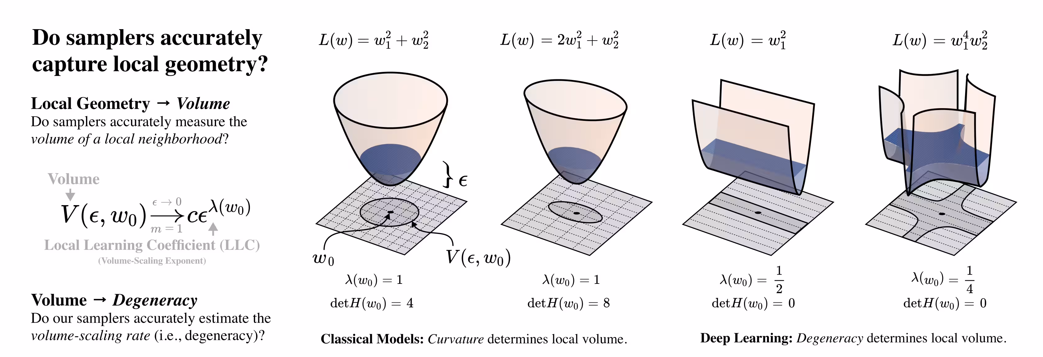
The premise is that the LLC captures something we’ve never had a good handle on: how “complex” or “singular” a solution is with respect to the geometry of its loss basin. Notionally, the LLC characterises the effective dimensionality (in some useful sense) of the loss landscape in overparameterized models such as neural networks.
Some arguments suggest the LLC is the “right” way to characterize this effective dimensionality, at least in the traditional setting where neural networks are viewed as Bayesian posteriors. In practice, that could mean:
- Comparing different minima from the same training run to understand which are “simpler.”1
- Tracking \(\lambda(w^*)\) across architectures, optimizers, or regularizers to see which design choices actually reduce effective complexity.
- Using it as a local diagnostic to interpret why two models with the same training loss generalize differently.
1 Needful formulae
Let \(L_n(w)\) be the empirical negative log‑likelihood and \(w^*\) a trained solution. Two equivalent forms drive everything, as far as I can tell:
- Local free energy (around \(w^*\))
\[ \begin{aligned} F_n(w^*,\gamma)&=-\log\!\int \exp\big(-n\,L_n(w)\big)\;\underbrace{\exp\!\big(-\tfrac{\gamma}{2}\|w-w^*\|^2\big)}_{\text{localizer}}\;dw\\ &=n\,L_n(w^*)\;+\;\lambda(w^*)\,\log n\;+\;o(\log n). \end{aligned} \]
- Operational (“WBIC‑style”) estimator
We choose the “hot” inverse temperature \(\beta^*=\tfrac{1}{\log n}\). I’m not sure why that particular temperature — I’m taking it on faith.
\[ p_{\beta,\gamma}(w\mid w^*)\ \propto\ \exp\!\Big(-n\beta\,L_n(w)-\tfrac{\gamma}{2}\|w-w^*\|^2\Big),\qquad \widehat{\lambda}(w^*)\;=\;n\beta^*\Big(\mathbb{E}_{p_{\beta^*,\gamma}}[L_n(w)]-L_n(w^*)\Big). \]
That’s the whole game: accurately approximate a single local expectation under a tempered, Gaussian‑tethered posterior.
2 HMC/MALA is hard at scale
I love HMC in moderate (say \(10^4\)) dimensions, but for LLC it runs into difficulties:
- Full‑batch acceptances. Any Metropolis‑corrected method needs accurate energy differences. In deep learning, that’s in principle a full pass over the dataset per proposal. With millions of parameters, even a modest trajectory is prohibitively expensive.
- Local restriction.
We don’t want the global posterior; we need a local one (that Gaussian “tether” around \(w^*\)). Enforcing locality inside standard HMC is finicky: it’s reject‑heavy, or we must hand‑craft reflective or soft constraints, which complicates tuning and implementation.No, I think I was wrong about that. The Gaussian localizer is part of the log‑density, so it’s just another term in the gradient, as far as I can see. We don’t need to do anything special. - Singular geometry. We expect directions around minima to be wildly anisotropic—many nearly flat, some very stiff. This should mix poorly because we’d spend a long time exploring the “wrong” directions — note, however, that the same is true of SGLD, and SGLD seems to work surprisingly well, so I might have bad intuition here.
3 SGLD
In practice, the workhorse is Stochastic Gradient Langevin Dynamics (SGLD). It looks almost like SGD, but with cleverly chosen Gaussian noise:
\[ w_{t+1} = w_t - \tfrac{\epsilon}{2}\,\widehat{\nabla} L_n(w_t)\;+\;\sqrt{\epsilon}\,\eta_t,\quad \eta_t \sim \mathcal N(0,I). \]
- The first term is the usual gradient step computed on a minibatch, so \(\widehat{\nabla} L_n\) is noisy.
- The second term is Gaussian noise, scaled to match the discretization of Langevin diffusion.
- Over many steps, the iterates approximate samples from a posterior distribution proportional to \(\exp(-nL_n(w))\).
Recall that for LLC estimation, we tweak two things:
- Tempering: we don’t want the true posterior; we want a hot version with inverse temperature \(\beta^*=1/\log n\). This means we multiply the gradient term by \(\beta^*\).
- Localization: we add a quadratic regularization term that pulls the chain towards the trained solution \(w^*\). This introduces an extra drift term \(-\tfrac{\epsilon}{2}\gamma(w_t-w^*)\). It looks like a Gaussian prior, but it isn’t — we invented it from the posterior.
So the update is:
\[ w_{t+1} = w_t - \tfrac{\epsilon}{2}\,\big(\beta^*\,\widehat{\nabla} L_n(w_t) + \gamma(w_t-w^*)\big)\;+\;\sqrt{\epsilon}\,\eta_t. \]
That’s the SGLD kernel we used in the LLC papers.
3.1 Preconditioned SGLD
One limitation of standard SGLD is that it makes isotropic moves: the Gaussian noise is spherical and the gradient step ignores differences in curvature across directions. In singular models, this makes us take tiny steps in stiff directions and explore slowly in flat ones.
A simple, affordable amelioration is to precondition. We introduce a positive-definite matrix \(A\) — think of the Adam quasi-curvature estimates, which give a diagonal approximation to \(A\). The update becomes:
\[ w_{t+1} = w_t - \tfrac{\epsilon}{2}\,A\big(\beta^*\,\widehat{\nabla} L_n(w_t) + \gamma(w_t-w^*)\big)\;+\;\xi_t,\quad \xi_t \sim \mathcal N(0,\,\epsilon A). \]
Now both the drift and the noise are scaled by \(A\). Intuitively, steps are larger in flat directions and smaller in sharp ones, with the noise scaled accordingly. This respects the desired invariant distribution (for constant \(A\)), makes exploration more efficient and preserves invariances such as weight rescaling in ReLU nets.
On paper, unadjusted Langevin with minibatches should make us nervous. In practice, SGLD tends to work because the LLC setup stacks the deck in our favour:
- It’s local. The quadratic \(\tfrac{\gamma}{2}\|w-w^*\|^2\) keeps the chain near \(w^*\). We don’t need to cross modes or map the whole loss landscape.
- It’s hot. \(\beta^*=1/\log n\) is small for big \(n\). Energy barriers are softened; local exploration is easier.
- It’s cheap. Minibatch gradients mean each step costs about an SGD step, so long chains are feasible.
- It’s tolerant. We only need \(\mathbb{E}[L_n(w)]\) to be accurate under the local law. We don’t require immaculate global mixing.
- It may be approximating nonparametric variational Bayes in some useful sense. See Hoffman and Ma (2020).
Intuitively, I think of the estimator as “explore the basin around \(w^*\) and see how quickly the loss rises.” If the basin is broad (singular/degenerate), the average loss near \(w^*\) barely increases and \(\widehat{\lambda}\) is small; if it’s sharp, the loss rises faster and \(\widehat{\lambda}\) is larger. SGLD seems smart at doing the poking, at least in the models I’ve tried.
We can show it works in practice for at least one model family: the deep linear network. There, we can test the estimates against ground truth. Indeed, the SGLD-based estimator matches the ground truth beautifully, even at big scales (hundreds of millions of parameters and datasets we can’t fully load into memory).
That’s surprising to me, and impressive. I think we have to be careful not to oversell it. DLNs are special: their singularities are structured in a way we can analyse, and the loss surface has symmetries that play nicely with the Gaussian driving noise.
In contrast, in nonlinear nets—with ReLU, GeLU, and friends—we don’t have an analytic ground truth for \(\lambda(w^*)\). All we can do is compare different estimators (SGLD vs MALA vs diagnostics), but they may share biases. It could be that SGLD is “working great” in DLNs precisely because they’re unusually well‑behaved, and that in truly nonlinear models the same algorithm is only approximately right.
So, while the DLN results give me confidence that the estimator isn’t nonsense, they shouldn’t be read as a general proof of correctness in deep nonlinear nets. This gap—we can’t validate LLC estimates in the models we actually care about—is, to me, concerning.
3.2 SGLD shortcomings
Note that there’s some unintuitive (to me) stuff going on here, even in tractable deep linear networks. The “landscape” has millions of dimensions, so “poking” in the right directions is hard, as it always is in high-dimensional models. There are various other things we might worry about:
- We aren’t actually using a great preconditioner. In practice we take Adam-style diagonal estimates, which assume our directions of interest are well captured by axis-aligned transformations; that seems plausible but far from certain. More sophisticated preconditioners (K-FAC, Shampoo, Muon) might help, but they’re more expensive and complicated.
- No universal guarantees in singular models. The standard SGLD convergence conditions (vanishing step sizes, Lyapunov tails) often fail for deep linear and modern nets. There are even clean examples where unadjusted Langevin diverges on light‑tailed targets.
- Discretization bias. With constant step sizes (what we actually use), we need strong diagnostics to keep bias small. In practice we rely on a MALA‑style acceptance‑probability diagnostic (not a real accept step) to tune the step size, and on long burn‑in until the minibatch‑loss trace flattens.
- Anisotropy hurts. Flat/stiff directions force tiny steps. Preconditioning (fixed diagonal, Fisher‑like) helps, but… is that enough? We know that in interesting models the local curvature matrix is not positive definite, so things are still not great.
- Hyperparameters matter. The localizer strength \(\gamma\) is a knob: too big and we drown out the likelihood geometry; too small and the chain can drift, even producing negative \(\widehat{\lambda}\).
- Finite‑\(n\) wrinkles. We evaluate at \(w^*\), which was trained on the same data we use inside the estimator. This works well empirically, but it’s not a theorem‑grade guarantee.
4 Variational Bayes
Instead of sampling from \(p_{\beta^*,\gamma}(w\mid w^*)\), we fit a local variational distribution \(q_\phi\) directly to it and use a plug-in estimate. We optimize the ELBO \[ \max_\phi\ \mathbb{E}_{q_\phi}\!\Big[-n\beta^* L_n(w) - \tfrac{\gamma}{2}\|w-w^*\|^2\Big] + \mathsf{H}(q_\phi), \] This lets us use all the standard tricks of stochastic-gradient variational inference (reparameterization, minibatches, etc). The LLC estimator is then \[ \widehat{\lambda}_{\text{VI}}(w^*) = n\beta^*\Big(\mathbb{E}_{q_\phi}[L_n(w)] - L_n(w^*)\Big). \] In general the bias obeys the identity \[ n\beta^*\big(\mathbb{E}_{q_\phi} L_n - \mathbb{E}_{p} L_n\big) + \tfrac{\gamma}{2}\Delta_2 = \mathrm{KL}(q_\phi \| p) + \mathsf{H}(q_\phi) - \mathsf{H}(p), \] with \(\Delta_2 = \mathbb{E}_{q_\phi}\|w - w^*\|^2 - \mathbb{E}_{p}\|w - w^*\|^2\).
5 Tempting alternatives I tried that don’t seem to work
I’ve kicked the tyres on several ideas that sounded like they should help. They did not.
5.1 Momentum SGMCMC (SGHMC / SGNHT)
Why I hoped it’d help. Momentum should cruise along flat manifolds and mix faster.
What goes wrong. For minibatch gradients, SGHMC requires a friction/noise correction matched to the gradient‑noise covariance. In deep nets, that noise can be heavy‑tailed and state‑dependent. The correction then becomes ill‑defined or expensive to estimate, and mis‑tuning yields a different stationary law. Net effect: we risk biasing the expectation that defines \(\widehat{\lambda}\), while adding tricky hyperparameters.
5.2 Twisted / optimally‑guided SMC
Why I hoped it’d help. SMC gives ESS diagnostics, tempering ladders, and MH‑corrected move steps (MALA/HMC) that avoid unadjusted‑Langevin pathologies.
What goes wrong. In very high dimension, we need excellent “twists” to avoid particle collapse. Twisted SMC works when there’s a trick that gives us good twists. Good twists aren’t obvious for arbitrary SLT models. Further, the moment we put accept/reject MALA/HMC inside SMC, we’re back to near full‑batch costs per particle. We can do it for small models (and it’s a good sanity check), but it’s not a scalable replacement.
5.3 Non‑Gaussian / Lévy noise (“spikier” SGLD)
Why I hoped it’d help. Heavy‑tailed jumps might traverse singular valleys faster.
What goes wrong. If we swap Gaussian noise for α‑stable jumps, then unless we also change the drift to the fractional counterpart and/or add an MH correction, the invariant law won’t be the tempered local posterior we need. If we add an MH step to fix it, we’re back to paying for full‑data accepts.
6 Where next
- The LLC estimator is local, hot, and tethered. Any method that respects those three features and keeps per‑step cost ≈ SGD can work. Right now, (preconditioned) SGLD seems to have a chance.
- Metropolis‑corrected moves are great…but at scale they’re not feasible. If we reintroduce full‑batch accepts (via HMC, heavy‑tailed MH, or SMC move steps), we lose the scalability that makes LLC estimation feasible.
- Changing the noise law doesn’t buy correctness. Lévy‑driven tricks either target the wrong distribution or demand accepts; neither is attractive here.
- Real open problems: provable control of discretization bias for constant‑stepsize, preconditioned SGLD in singular models; principled selection of the localizer strength \(\gamma\); and geometry‑aware preconditioners that preserve the estimator’s invariances without expensive curvature estimation.
7 Potential angles of attack.
🚧TODO🚧: write these out so they make sense to other people.
- Transdimensional Hironaka moves
- Basin-friendly preconditioning estimators
- Online updates
8 Incoming
Connection to Muon and other normalizer approaches that give us “free” preconditioning and other nice things.
Will Microcanonical LMC do better?
UPDATE: In my little prototype, MCLMC is very fast but doesn’t seem to converge.
honglu2875/hironaka: A utility package for Hironaka game of local resolution of singularities
Eleuther’s local volume measurement seems related: Research Update: Applications of Local Volume Measurement | EleutherAI Blog
9 References
Footnotes
We need to be careful about what actually counts as a minimum in this setting — did we even converge, and what would that mean?↩︎