Optimal transport inference
I feel the earth mover under my feet, I feel the ψ tumbling down, I feel my heart start to trembling, whenever you’re around (my barycentre)
2021-03-16 — 2023-05-03
Wherein optimal-transport based inference is surveyed, and practical expedients such as the estimation of Monge transport maps or minibatched Sinkhorn approximations for Wasserstein losses are indicated.
Doing inference where the probability metric measuring discrepancy between some target distribution and the implied inferential distribution is an optimal-transport one. Frequently intractable, but neat when we can get it. Sometimes we might get there by estimating the (gradients of) an actual OT loss, or even the transport maps implying that loss.
Placeholder/grab bag.
TODO: should we break this into discrete-state and continuous-state cases? Machinery looks different.
1 NNs
Wasserstein GANs and OT Gans (Salimans et al. 2018) are argued to do an approximate optimal transport inference, indirectly.
2 Surprise connection to matrix factorisation
Non-negative matrix factorisation via OT is a thing, e.g. in topic modeling (Huynh, Zhao, and Phung 2020; Zhao et al. 2020).
3 Via Fisher distance
See e.g. (J. H. Huggins et al. 2018b, 2018a) for a particular Bayes posterior approximation using OT and fisher distance.
4 Minibatched
Daniel Daza in Approximating Wasserstein distances with PyTorch touches upon Fatras et al. (2020):
Optimal transport distances are powerful tools to compare probability distributions and have found many applications in machine learning. Yet their algorithmic complexity prevents their direct use on large scale datasets. To overcome this challenge, practitioners compute these distances on minibatches i.e., they average the outcome of several smaller optimal transport problems. We propose in this paper an analysis of this practice, which effects are not well understood so far. We notably argue that it is equivalent to an implicit regularization of the original problem, with appealing properties such as unbiased estimators, gradients and a concentration bound around the expectation, but also with defects such as loss of distance property.
5 Linearized embedding
Noted in Bai et al. (2023) via Cheng-Soon Ong:
Comparing K (probability) measures requires the pairwise calculation of transport-based distances, which, despite the significant recent computational speed-ups, remains to be relatively expensive. To address this problem, W. Wang et al. (2013) proposed the Linear Optimal Transport (LOT) framework, which linearizes the 2-Wasserstein distance utilising its weak Riemannian structure. In short, the probability measures are embedded into the tangent space at a fixed reference measure (e.g., the measures’ Wasserstein barycenter) through a logarithmic map. The Euclidean distances between the embedded measures then approximate the 2-Wasserstein distance between the probability measures. The LOT framework is computationally attractive as it only requires the computation of one optimal transport problem per input measure, reducing the otherwise quadratic cost to linear. Moreover, the framework provides theoretical guarantees on convexifying certain sets of probability measures […], which is critical in supervised and unsupervised learning from sets of probability measures.
6 Tools
6.1 OTT
Optimal Transport Tools (OTT) (Cuturi et al. 2022), a toolbox for all things Wasserstein (documentation):
The goal of OTT is to provide sturdy, versatile and efficient optimal transport solvers, taking advantage of JAX features, such as JIT, auto-vectorization and implicit differentiation.
A typical OT problem has two ingredients: a pair of weight vectors
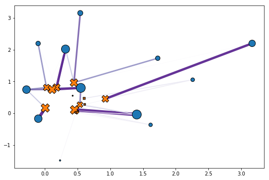
aandb(one for each measure), with a ground cost matrix that is either directly given, or derived as the pairwise evaluation of a cost function on pairs of points taken from two measures. The main design choice in OTT comes from encapsulating the cost in aGeometryobject, and [bundling] it with a few useful operations (notably kernel applications). The most common geometry is that of two clouds of vectors compared with the squared Euclidean distance, as illustrated in the example below:
import jax
import jax.numpy as jnp
from ott.tools import transport
# Samples two point clouds and their weights.
rngs = jax.random.split(jax.random.PRNGKey(0),4)
n, m, d = 12, 14, 2
x = jax.random.normal(rngs[0], (n,d)) + 1
y = jax.random.uniform(rngs[1], (m,d))
a = jax.random.uniform(rngs[2], (n,))
b = jax.random.uniform(rngs[3], (m,))
a, b = a / jnp.sum(a), b / jnp.sum(b)
# Computes the couplings via Sinkhorn algorithm.
ot = transport.solve(x, y, a=a, b=b)
P = ot.matrix
The call to
sinkhornabove works out the optimal transport solution by storing its output. The transport matrix can be instantiated using those optimal solutions and theGeometryagain. That transport matrix links each point from the first point cloud to one or more points from the second, as illustrated below.To be more precise, the
sinkhornalgorithm operates on theGeometry, taking into account weightsaandb, to solve the OT problem, produce a named tuple that contains two optimal dual potentialsfandg(vectors of the same size asaandb), the objectivereg_ot_costand a log of theerrorsof the algorithm as it converges, and aconvergedflag.
6.2 POT
POT: Python Optimal Transport (Rémi Flamary et al. 2021)
This open source Python library provides several solvers for optimization problems related to Optimal Transport for signal, image processing and machine learning.
Website and documentation: https://PythonOT.github.io/
Source Code (MIT): https://github.com/PythonOT/POT
POT provides the following generic OT solvers (links to examples):
- OT Network Simplex solver for the linear program/ Earth Movers Distance.
- Conditional gradient and Generalized conditional gradient for regularized OT.
- Entropic regularization OT solver with Sinkhorn Knopp Algorithm, stabilized version, greedy Sinkhorn and Screening Sinkhorn.
- Bregman projections for Wasserstein barycenter, convolutional barycenter and unmixing.
- Sinkhorn divergence and entropic regularization OT from empirical data.
- Debiased Sinkhorn barycenters Sinkhorn divergence barycenter
- Smooth optimal transport solvers (dual and semi-dual) for KL and squared L2 regularizations.
- Weak OT solver between empirical distributions
- Non regularized Wasserstein barycenters with LP solver (only small scale).
- Gromov-Wasserstein distances and GW barycenters (exact and regularized), differentiable using gradients from Graph Dictionary Learning
- Fused-Gromov-Wasserstein distances solver and FGW barycenters
- Stochastic solver and differentiable losses for Large-scale Optimal Transport (semi-dual problem and dual problem)
- Sampled solver of Gromov Wasserstein for large-scale problem with any loss functions
- Non regularized free support Wasserstein barycenters.
- One dimensional Unbalanced OT with KL relaxation and barycenter \[10, 25\]. Also exact unbalanced OT with KL and quadratic regularization and the regularization path of UOT
- Partial Wasserstein and Gromov-Wasserstein (exact and entropic formulations).
- Sliced Wasserstein \[31, 32\] and Max-sliced Wasserstein that can be used for gradient flows.
- Graph Dictionary Learning solvers.
- Several backends for easy use of POT with Pytorch/jax/Numpy/Cupy/Tensorflow arrays.
POT provides the following Machine Learning related solvers:
- Optimal transport for domain adaptation with group lasso regularization, Laplacian regularization and semi supervised setting.
- Linear OT mapping and Joint OT mapping estimation.
- Wasserstein Discriminant Analysis (requires autograd + pymanopt).
- JCPOT algorithm for multi-source domain adaptation with target shift.
Some other examples are available in the documentation.
6.3 GeomLoss
The GeomLoss library provides efficient GPU implementations for:
- Kernel norms (also known as Maximum Mean Discrepancies).
- Hausdorff divergences, which are positive definite generalizations of the Chamfer-ICP loss and are analogous to log-likelihoods of Gaussian Mixture Models.
- Debiased Sinkhorn divergences, which are affordable yet positive and definite approximations of Optimal Transport (Wasserstein) distances.
It is hosted on GitHub and distributed under the permissive MIT license.
GeomLoss functions are available through the custom PyTorch layers
SamplesLoss,ImagesLossandVolumesLosswhich allow you to work with weighted point clouds (of any dimension), density maps and volumetric segmentation masks.
7 Incoming
Rigollet and Weed (2018):
We give a statistical interpretation of entropic optimal transport by showing that performing maximum-likelihood estimation for Gaussian deconvolution corresponds to calculating a projection with respect to the entropic optimal transport distance.
Thomas Viehmann, An efficient implementation of the Sinkhorn algorithm for the GPU is a Pytorch CUDA extension (Viehmann 2019)
Marco Cuturi’s course notes on OT include a 400 page slide deck.


