Orthonormal and unitary matrices
Energy preserving operators, generalized rotations
2019-10-22 — 2025-05-22
In which I think about parameterisations and implementations of finite-dimensional energy-preserving operators, a.k.a. orthonormal matrices. A type of tool in the linear feedback process library, closely related to stability in linear dynamical systems, since every orthonormal matrix is the forward operator of an energy-preserving system, which is an edge case for certain natural types of stability. Also important in random low-dimensional projections.
Uses include maintaining stable gradients in recurrent neural networks (Arjovsky, Shah, and Bengio 2016; Jing et al. 2017; Mhammedi et al. 2017) and efficient invertible normalising flows (van den Berg et al. 2018; Hasenclever, Tomczak, and Welling 2017). Also, parameterising stable Multi-Input-Multi-Output (MIMO) delay networks in signal processing. Probably other stuff too.
Terminology: Some writers refer to orthogonal matrices (but I prefer that to mean matrices where the columns are not necessarily 2-norm 1), and some refer to unitary matrices, which implies that the matrix is over the complex field instead of the reals but is basically the same from my perspective.
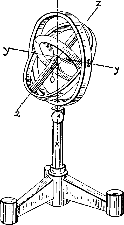
We also might want to consider the implied manifolds upon which these objects live, the Stiefel manifold. Formally, the Stiefel manifold
Finding an orthonormal matrix is equivalent to choosing a finite orthonormal basis, so any way we can parameterise such a basis gives us an orthonormal matrix.
NB the normalisation implies that the basis for an
TODO: discuss rectangular and square orthogonal matrices.
1 Take the QR decomposition
HT Russell Tsuchida for pointing out that the
The construction of the QR decomposition Householder reflections is, Wikipedia reckons,
2 Other decompositions?
We can get something which looks similar via the Lanczos algorithm, which handles warm starts, finding
Question: do the spectral radius upper-bounds of NO-BEARS (Lee et al. 2019; Zhu et al. 2020), give us a pointer towards another method for finding such matrices? (HT Dario Draca for mentioning this.) I think that gets us something “sub”-orthonormal in general, since it will upper-bound the determinant. Or something.
3 Iterative normalising
Have a nearly orthonormal matrix? van den Berg et al. (2018) gives a contraction towards a nearby orthonormal matrix:
4 Perturbing an existing orthonormal matrix
Unitary transforms map unitary matrices to unitary matrices. We can even start from the identity matrix and perturb it to traverse the space of unitary matrices.
4.1 Householder reflections
We can apply successive reflections about hyperplanes, the so-called Householder reflections, to an orthonormal matrix to construct a new one. For a unit vector
4.2 Givens rotation
One obvious method for constructing unitary matrices is composing Givens rotations, which are atomic rotations about 2 axes.
A Givens rotation is represented by a matrix of the form
5 Cayley map
The Cayley map maps the skew-symmetric matrices to the orthogonal matrices of positive determinant, and parameterising skew-symmetric matrices is easy; just take the upper triangular component of some matrix and flip/negate it. This still requires a matrix inversion in general, AFAICS.
6 Exponential map
The exponential map (Golinski et al., 2019). Given a skew-symmetric matrix A, i.e. a
matrix such that , the matrix exponential is always an orthogonal matrix with determinant 1. Moreover, any orthogonal matrix with determinant 1 can be written this way. However, computing the matrix exponential takes in general time, so this parameterisation is only suitable for small-dimensional data.
7 Parametric sub-families
Citing MATLAB, Nick Higham gives the following two parametric families of orthonormal matrices. These are clearly far from covering the whole space of orthonormal matrices.
8 Newton-Schulz iteration
Noted at SGD at scale, in Deriving Muon (Bernstein and Newhouse 2024b)
Some papers using it here:
(Bernstein et al. 2020; Bernstein and Newhouse 2024b, 2024a; HighamMatrix?; Large et al. 2024; Yang, Simon, and Bernstein 2023)
- The modula.systems Newton-Schulz docs are best for now I think
9 Structured
Orthogonal convolutions? TBD
10 Random distributions over
I wonder what the distribution of orthonormal decompositions matrices is for some, say, matrix with independent standard Gaussian entries? Nick Higham has the answer, in his compact introduction to random orthonormal matrices. A uniform, rotation-invariant distribution is given by the Haar measure over the group of orthogonal matrices. He also gives the construction for drawing them by random Householder reflections derived from random standard normal vectors. See random rotations.
11 Hurwitz matrix
A related concept. Hurwitz matrices define asymptotically stable systems of ODEs, which is not the same as conserving the energy of a vector. Also they pack the transfer function polynomial in a weird way.