The denoising diffusion SDE
Stochastic diffusions that are reversible in a computationally useful sense
2023-12-09 — 2025-11-08
Wherein the Forward Diffusion Is Described and the Reverse‑time SDE Is Shown to Require the Score, the Gradient of the Log Density, Which Is Approximated by a Time‑conditioned Neural Network Trained by Denoising, Enabling Sampling From Complex Multimodal Targets.
Sample from tricky distributions via the clever use of stochastic differential equations. Diffusion models use time-evolving stochastic differential equations to transform between distributions we have and those we want. They were made famous by neural diffusions and score diffusion more generally.
1 From the score matching side
In score matching we saw how to learn an unnormalized model by training its score function — the gradient of the log density — rather than the density directly. That trick — matching scores instead of probabilities — was a conceptual leap: we could sidestep the intractable partition function and still fit energy-based models.
But in denoising score matching we only added a single level of Gaussian noise. What if, instead of one noisy layer, we gradually destroyed structure in the data, adding more and more noise until everything became pure Gaussian randomness — and then trained a model to reverse that process?
Why, then we would have invented denoising diffusion models.
1.1 Multi-scale denoising diffusion
In standard score matching, we learn: \[ s_\theta(y) \approx \nabla_y \log p_\text{data}(y) \] by perturbing samples with small Gaussian noise and predicting the direction back to the clean data.
In diffusion models, we take this to the limit: we don’t add one small noise, but a continuous sequence of them. Let \(y_0\) be a clean data point. We define a forward process that gradually corrupts the data point (for intuition, we first write a VE (variance-exploding) forward SDE with \(b \equiv 0\); below we switch to VP): \[ \mathrm{d} y_t = \sqrt{\beta_t}\, \mathrm{d} W_t, \] where \(W_t\) is a Wiener process and \(\beta_t\) controls the noise rate.
As \(t \to 1\), with a VP schedule the law approaches \(\mathcal{N}(0, I)\); for VE the variance grows large unless we rescale. This process defines a diffusion — it literally diffuses the data distribution into noise.
If we can simulate the forward diffusion (data → noise), can we go backward (noise → data)?
Formally, the reverse-time SDE (with time running backward) is: \[ \mathrm{d} y_t = \left[ b(t, y_t) - a(t) \nabla_{y_t} \log p_t(y_t) \right] \mathrm{d}t + \sigma(t)\, \mathrm{d}\bar W_t, \] where \(a(t) = \sigma(t)\sigma(t)^\top\), \(p_t\) are the marginal distributions at time \(t\), and the key term \(\nabla_{y_t} \log p_t(y_t)\) is — again — the score.
To integrate backward, we need to know the score at every noise level \(t\). We can’t observe it directly any more than we could in the vanilla score-matching case, but we can train a neural network \(s_\theta(y_t, t)\) to approximate it.
How that works: For each \(t\), we perturb the data with variance corresponding to \(t\), \[ \tilde y_t = \sqrt{\alpha_t} y_0 + \sqrt{1-\alpha_t}\,\varepsilon, \quad \varepsilon\sim\mathcal N(0,I), \] We train \(s_\theta(\tilde y_t, t)\) to predict the conditional corruption score \(-\varepsilon/\sqrt{1-\alpha_t}\). By \(\nabla_{y_t} \log p_t(y_t) = \mathbb{E}_{y_0|y_t}[\nabla_{y_t} \log p(y_t|y_0)]\), we recover the marginal score in expectation: \[ s_\theta(\tilde y_t, t) \approx \nabla_{y_t} \log p_t(\tilde y_t). \]
So, diffusion training is multi-scale denoising score matching.
1.2 Multi-scale Fisher divergence
We can also interpret diffusion training as minimizing a time-weighted version of the Fisher divergence: \[ \mathcal L =\mathbb E_{t\sim[0,1]} \mathbb E_{y_0,\varepsilon} \big[ \lambda(t)\, \|s_\theta(\tilde y_t, t) + \tfrac{\varepsilon}{\sqrt{1-\alpha_t}}\|^2 \big]. \]
Train a time-indexed score network \(s_\theta(x,t) \approx \nabla_x \log p_t(x)\) by denoising Gaussian-corrupted data at many noise levels. Sampling integrates the reverse-time SDE \[ dZ_t = \left[ b(t,Z_t) - a(t) \nabla_x \log p_t(Z_t) \right] dt + \sigma(t) \, d\bar{W}_t \] from noise back to data, replacing the unknown score with \(s_\theta\) at sampling time.
(In the derivations below, we use \(z\) as the state variable and \(p_\tau (z)\) for marginal densities. From here on I write \(Z_\tau\) for the state; it’s the same object previously denoted \(y_t\).)
2 As time-reversal of noising processes
Conceptually, denoising diffusions require two pieces of infrastructure:
- Forward Process (“Diffusion”): Gradually adds noise to the data, transforming it into a known reference distribution (typically \(\mathcal{N}(0,I)\)).
- Reverse Process (“Denoising”): Removes the noise, transforming the reference distribution back into the target data distribution.
It’s not surprising that we can set up the forward process. The surprising thing is that the reverse process also works—that’s a neat result from the theory of SDEs.
Forward SDE (\(t \in [0,T]\)): \[ dZ_t = b(t, Z_t)\, dt + \sigma(t)\, dW_t \] where \(a(t) = \sigma(t)\sigma(t)^\top\) is the diffusion matrix.
Reverse-time SDE (with time running backward, \(t \in [T,0]\)): \[ dZ_t = \left[b(t, Z_t) - a(t)\nabla_z \log p_t(Z_t)\right] dt + \sigma(t)\, d\overleftarrow{W}_t \]
Equivalently, with forward-running “reverse clock” \(s := T - t\) (so \(s \in [0,T]\)): \[ d\tilde{Z}_s = \left[b(T{-}s, \tilde{Z}_s) - a(T{-}s)\nabla_z \log p_{T-s}(\tilde{Z}_s)\right] ds + \sigma(T{-}s)\, d\overleftarrow{W}_s \]
Rather than just taking the neat off-the-rack results from the literature, I work through the derivation myself in the hope that it will help me understand it better.
2.1 Setup
The forward SDE characterises the forward process, describing how we add noise to the data until it matches the reference distribution. We consider a stochastic differential equation (SDE) of the form
\[ dZ_{\tau} = b(\tau, Z_{\tau}) \, d\tau + \sigma(\tau) \, dW_{\tau} \tag{1}\]
where we define the diffusion matrix \(a(\tau) = \sigma(\tau)\sigma(\tau)^\top\) (which reduces to \(\sigma^2(\tau)\) in the scalar case).
- \(Z_{\tau}\): State at time \(\tau \in [0, 1]\).
- \(b(\tau, z)\): Drift coefficient (may depend on state \(z\)).
- \(\sigma(\tau)\): Diffusion coefficient.
- \(dW_{\tau}\): Increment of a standard Wiener process (Brownian motion).
To reverse the diffusion process and construct the reverse-time (denoising) process, we use the backward SDE. To make this guy go we have to introduce some extra notation. Let \(p_{\tau}(z)\) denote the marginal density of \(Z_{\tau}\) at time \(\tau\). The backward SDE (interpreted with time running backward) is:
\[ \begin{aligned} dZ_{\tau} &= \left[ b(\tau, Z_{\tau}) - a(\tau) \nabla_z \log p_{\tau}(Z_{\tau}) \right] \, d\tau + \sigma(\tau) \, d\overleftarrow{W}_{\tau} \\ &= \tilde{b}(\tau, Z_{\tau}) \, d\tau + \sigma(\tau) \, d\overleftarrow{W}_{\tau} \end{aligned} \tag{2}\]
- \(\nabla_z \log p_{\tau}(Z_{\tau})\): Score function of the marginal density at time \(\tau\).
- \(\tilde{b}(\tau, z) = b(\tau, z) - a(\tau) \nabla_z \log p_{\tau}(z)\): Adjusted drift term.
- \(d\overleftarrow{W}_{\tau}\): A Brownian motion adapted to the backward filtration. Note: you should not identify its increment with \(-dW\) pathwise.
What in blazes happened there? Where did this \(p\) come from? What even is this backward Wiener process? Why are these terms like they are? etc. There is a claim about Fokker-Planck equations that is traditional, but it is not very intuitive, and introduces some heavy machinery which doesn’t really build intuition. So I moved that to the end.
Let us understand this in a more intuitive way, i.e., by being dumb about it and seeing what does not work.
We run into ALL KINDS OF CRAZY when it comes to working out which direction time is running here. I’ve put a negative sign in front of the drift term in the backward SDE to make it look like the forward SDE, but this is a slightly weird way of doing things, because it implies that time is running forward, rather than backward, and we are looking at a backward SDE. I think I am being consistent about this, but feel free to call me out if I am not. Alternatively, you might want to read this post upside-down.
2.2 Let us discretize
OK, first simplification, we consider the Euler-Maruyama discretization of the forward SDEs Equation 1, and take that as ground-truth for now. In this one, we ignore continuous time but think about small time steps \(\Delta \tau\) over which behaviour is approximately linear. Throughout, \(I\) denotes the identity matrix in \(d\) dimensions.
With this discretization, let us think about the distribution of \(Z_{\tau}\) given \(Z_{\tau{+}\Delta\tau}\). For a small step \(\Delta\tau\),
\[ Z_{\tau+\Delta \tau} = Z_{\tau} + b(\tau, Z_{\tau}) \, \Delta\tau + \sigma(\tau) \Delta W_{\tau} \tag{3}\]
From here to §Markov kernels we work in 1D for notational simplicity; in higher dimensions replace \(a(\tau)\) by the matrix \(a(\tau)=\sigma(\tau)\sigma(\tau)^\top\) and use the quadratic form \((z'-z)^\top a^{-1} (z'-z)\) in place of \(\|z'-z\|^2 / a\).
The forward transition kernel \(p_{\text{forward}}(z_{\tau{+}\Delta\tau} | z_{\tau})\) is the probability density of \(Z_{\tau{+}\Delta\tau}\) given \(Z_{\tau}=z_{\tau}\). We have
\[ Z_{\tau{+}\Delta\tau} | Z_{\tau}=z_{\tau} \sim \mathcal{N}\bigl(z_{\tau} + b(\tau,z_{\tau})\Delta\tau,\; a(\tau)\Delta\tau\bigr). \]
Hence, the forward transition kernel is \[ p_{\text{forward}}(z_{\tau{+}\Delta\tau}|z_{\tau}) = \frac{\exp\left(-\frac{\| z_{\tau{+}\Delta\tau}-z_{\tau}-b(\tau,z_{\tau})\Delta\tau \|^2}{2a(\tau)\Delta\tau}\right)}{\sqrt{2\pi a(\tau)\Delta\tau}}. \tag{4}\]
Discretization of the backward SDE Equation 2 proceeds similarly. The Euler-Maruyama discretization gives:
\[ Z_{\tau} = Z_{\tau{+}\Delta\tau} + \left[b(\tau{+}\Delta\tau, Z_{\tau{+}\Delta\tau}) - a(\tau{+}\Delta\tau)\nabla_z \log p_{\tau{+}\Delta\tau}(Z_{\tau{+}\Delta\tau})\right]\Delta\tau + \sigma(\tau{+}\Delta\tau)\Delta\overleftarrow{W}_{\tau}. \tag{5}\]
Since \(\Delta\overleftarrow{W}_{\tau} \sim \mathcal{N}(0,\Delta\tau I)\), the conditional distribution \(Z_{\tau}|Z_{\tau{+}\Delta\tau}=z_{\tau{+}\Delta\tau}\) is also Gaussian.
Hence the backward transition kernel is \[ p_{\text{backward}}(z_{\tau}|z_{\tau{+}\Delta\tau}) = \mathcal{N}\left( z_{\tau} \, \bigg| \, z_{\tau{+}\Delta\tau} - \left[ b(\tau{+}\Delta\tau, z_{\tau{+}\Delta\tau}) - a(\tau{+}\Delta\tau) \nabla_z \log p_{\tau{+}\Delta\tau}(z_{\tau{+}\Delta\tau}) \right]\Delta\tau, \; a(\tau{+}\Delta\tau)\Delta\tau \right). \tag{6}\]
Writing it this way was a chaotic move, but it gives us the tools to play with these distributions and see what happens. Also it puts lots of Greek letters on the page, which makes us look clever.
2.3 Pathwise Euler-Maruyama update
The following analysis attempts a pathwise interpretation of time reversal, but this approach is incorrect. Round-trip inversion is a statement about transition kernels and marginals, not about canceling a particular sample path. The reverse Brownian motion is independent of the forward increment, not its negative. But I needed to work this out by hand to persuade myself, and I found this blatant error helpful, so you might too.
Now, let us consider a single path of the forward and backward SDEs. Let us see what happens when we apply the forward and backward steps to a single path.
We consider a variate \(Z_{\tau}'\), which arises from applying the forward then backward steps to a variate \(Z_{\tau}\), i.e. \[ \begin{aligned} Z_{\tau}' &= Z_{\tau{+}\Delta\tau} - \tilde{b}(\tau{+}\Delta\tau, Z_{\tau{+}\Delta\tau})\Delta\tau + \sigma(\tau{+}\Delta\tau)\Delta\overleftarrow{W}_{\tau}\\ &= Z_{\tau} + b(\tau, Z_{\tau}) \, \Delta\tau + \sigma(\tau) \Delta W_{\tau} - \tilde{b}(\tau{+}\Delta\tau, Z_{\tau{+}\Delta\tau})\Delta\tau + \sigma(\tau{+}\Delta\tau)\Delta\overleftarrow{W}_{\tau}\\ &= Z_{\tau} + b(\tau, Z_{\tau}) \, \Delta\tau + \sigma(\tau) \Delta W_{\tau} - \left[ b(\tau{+}\Delta\tau, Z_{\tau{+}\Delta\tau}) - a(\tau{+}\Delta\tau) \nabla_z \log p_{\tau{+}\Delta\tau}(Z_{\tau{+}\Delta\tau}) \right]\Delta\tau + \sigma(\tau{+}\Delta\tau)\Delta\overleftarrow{W}_{\tau}. \end{aligned} \]
The following reasoning is incorrect: One might naively suppose that “reversibility” means \(\Delta\overleftarrow{W}_{\tau} = -\Delta W_{\tau}\) pathwise. This is false: \(\Delta\overleftarrow{W}_{\tau}\) is an independent Brownian increment, not the negative of \(\Delta W_{\tau}\). Nevertheless, let us see where this faulty reasoning leads.
Under this incorrect assumption
\[ \begin{aligned} Z_{\tau}' &= Z_{\tau} + b(\tau, Z_{\tau}) \, \Delta\tau + \sigma(\tau) \Delta W_{\tau} - \left[ b(\tau{+}\Delta\tau, Z_{\tau{+}\Delta\tau}) - a(\tau{+}\Delta\tau) \nabla_z \log p_{\tau}(Z_{\tau}) \right]\Delta\tau + \sigma(\tau{+}\Delta\tau)\Delta\overleftarrow{W}_{\tau}\\ &= Z_{\tau} + (b(\tau, Z_{\tau}) - b(\tau{+}\Delta\tau, Z_{\tau{+}\Delta\tau}))\Delta\tau + a(\tau{+}\Delta\tau) \nabla_z \log p_{\tau}(Z_{\tau{+}\Delta\tau}) \Delta\tau + (\sigma(\tau) - \sigma(\tau{+}\Delta\tau))\Delta W_{\tau}. \end{aligned} \]
So that doesn’t look like it will return a given point to its original state, in general.
Even if we think the equations are stationary, it is unclear why the bias term would cancel, and we might not be persuaded that the diffusion term would go to zero. \[ \begin{aligned} Z_{\tau}' &= Z_{\tau} + b(Z_{\tau}) \, \Delta\tau + \sigma \Delta W_{\tau} - \left[ b(Z_{\tau{+}\Delta\tau}) - \sigma^2 \nabla_z \log p_{\tau}(Z_{\tau}) \right]\Delta\tau + \sigma\Delta\overleftarrow{W}_{\tau}\\ &= Z_{\tau} + (b(Z_{\tau}) - b(Z_{\tau{+}\Delta\tau}))\Delta\tau + \sigma^2 \nabla_z \log p_{\tau}(Z_{\tau{+}\Delta\tau}) \Delta\tau + (\sigma - \sigma)\Delta W_{\tau}\\ &= Z_{\tau} + (b(Z_{\tau}) - b(Z_{\tau{+}\Delta\tau}))\Delta\tau + \sigma^2 \nabla_z \log p_{\tau}(Z_{\tau{+}\Delta\tau}) \Delta\tau. \end{aligned} \] (In this stationary 1D example, \(a = \sigma^2\).)
Under this (wrong) assumption, the terms still do not cancel pathwise. This illustrates why time reversal is about transition kernels and marginal densities, not individual sample trajectories.
2.4 Markov kernels
OTOH, we could wonder if the marginal density \(p_\tau (z)\) is preserved by the application of the forward step and the backward step in turn. Let’s see how to approach this.
The resulting probability density arises from the double integral,
\[ p(Z_{\tau}' | Z_{\tau} = z_{\tau}) = \int p_{\text{backward}}(Z_{\tau}' | Z_{\tau{+}\Delta\tau} = z_{\tau{+}\Delta\tau}) \, p_{\text{forward}}(Z_{\tau{+}\Delta\tau} = z_{\tau{+}\Delta\tau} | Z_{\tau} = z_{\tau}) \, dz_{\tau{+}\Delta\tau}. \]
This integral represents the composition of the forward transition from \(z_{\tau}\) to \(z_{\tau{+}\Delta\tau}\) followed by the backward transition from \(z_{\tau{+}\Delta\tau}\) to \(Z_{\tau}'\). Our goal is to evaluate this integral to understand how applying the forward and backward steps affects the original state \(z_{\tau}\).
We know from the theory of time-reversed Markov processes that the backward kernel can be expressed in terms of the forward kernel and the ratio of marginals. This relationship arises from Bayes’ rule applied to transition densities:
\[ p_{\text{backward}}(z_{\tau}|z_{\tau{+}\Delta\tau}) = \frac{p_{\text{forward}}(z_{\tau{+}\Delta\tau}|z_{\tau})\,p_{\tau}(z_{\tau})}{p_{\tau{+}\Delta\tau}(z_{\tau{+}\Delta\tau})}. \]
To ensure the backward step is the inverse of the forward step (in an infinitesimal sense), the drift \(\tilde{b}\) must be chosen so that this relationship holds. In fact, identifying:
\[ \tilde{b}(\tau,z) = b(\tau,z) - a(\tau)\nabla_z \log p_{\tau}(z) \]
is exactly the condition that makes this inverse relationship work. This ensures that the composition of forward and backward kernels returns the marginal to first order:
\[ \int p_{\text{backward}}(z|z') \, p_{\text{forward}}(z'|x) \, dz' \to \delta(z-x) \quad \text{to first order as } \Delta\tau \to 0. \]
Equivalently, when applied to densities, the round-trip preserves the marginal:
\[ \int p_{\text{backward}}(z|z') \left[\int p_{\text{forward}}(z'|x) p_{\tau}(x) \, dx\right] dz' \to p_{\tau}(z) \quad \text{to first order as } \Delta\tau \to 0. \]
This operator identity means that a forward step followed by a backward step returns the distribution close to where it started, consistent with the idea of time reversal.
We consider a small time interval \(\Delta \tau\) and show that the forward and backward steps are inverses of each other. I.e. take the Euler-Maruyama discretization as given, and ignore questions about infinite limits and so on. The forward and backward steps are each some linear operation on some Gaussian noise.
Forward Step:
Starting from \(Z_{\tau}\), the forward SDE updates \(Z_{\tau + \Delta \tau}\):
\[ Z_{\tau + \Delta \tau} = Z_{\tau} + b(\tau, Z_{\tau}) \Delta \tau + \sigma(\tau) \Delta W_{\tau} \]
Backward Step:
Starting from \(Z_{\tau + \Delta \tau}\), the backward SDE updates \(Z_{\tau}\):
\[ Z_{\tau} = Z_{\tau{+}\Delta\tau} + \tilde{b}(\tau{+}\Delta\tau, Z_{\tau{+}\Delta\tau}) \Delta \tau + \sigma(\tau{+}\Delta\tau) \Delta \overleftarrow{W}_{\tau} \]
If you are like me, you did not find that especially helpful for intuition-building, which is probably why they do not bother with it in typical blog posts about score diffusions. Let us try to make it concrete by actually working through the steps of the reverse SDE.
Backward Step plus forward step:
We can substitute the forward step into the backward step to get a concrete expression for the concatenation of these steps. Since this is a Gaussian we can think about the evolution in terms of the mean and variance of the distribution.
Let us fix a path of \(Z_{\tau}=z_{\tau}\) and consider the evolution of the distribution, i.e.
\[ \begin{aligned} (Z_{\tau + \Delta \tau}\mid Z_{\tau}=z_{\tau} ) &= z_{\tau} + b(\tau, z_{\tau}) \Delta \tau + \sigma(\tau) \Delta W_{\tau} \end{aligned} \]
- (Counterfactual; not true) If \(\Delta W_{\tau}\) and \(\Delta \overleftarrow{W}_{\tau}\) were such that \(\Delta \overleftarrow{W}_{\tau} = -\Delta W_{\tau}\), then the stochastic terms would cancel out.
- The score function \(\nabla_z \log p_{\tau}(Z_{\tau})\) ensures that the drift terms are adjusted appropriately.
\[ Z_{\tau} = Z_{\tau + \Delta \tau} + \left[ -b(\tau+\Delta\tau, Z_{\tau + \Delta \tau}) + a(\tau+ \Delta \tau) \nabla_z \log p_{\tau + \Delta \tau}(Z_{\tau + \Delta \tau}) \right] \Delta \tau + \sigma(\tau{+}\Delta\tau) \Delta \overleftarrow{W}_{\tau+ \Delta \tau} \]
(This is the correct reverse update; note \(\Delta\overleftarrow{W}\) is independent of \(\Delta W\).)
3 Practical example
Below is an example of numerically simulating forward and backward SDEs using JAX. We use a standard Variance Preserving (VP) diffusion that transforms data to a Gaussian.
Above I illustrated the drift-free (VE) case for intuition; below I switch to the VP SDE used in DDPMs for the concrete simulation.
First, let’s import the necessary libraries.
3.1 SDE Coefficients
We use a simple Variance Preserving (VP) forward SDE: \[ dZ_{\tau} = -\frac{\beta(\tau)}{2} Z_{\tau} d\tau + \sqrt{\beta(\tau)} dW_{\tau} \]
with linear noise schedule \(\beta(\tau) = \beta_{\min} + (\beta_{\max} - \beta_{\min})\tau\).
Code
# Noise schedule parameters
beta_min = 0.1
beta_max = 20.0

def beta_tau(tau):
    return beta_min + (beta_max - beta_min) * tau

def b_tau(tau, z):
    return -0.5 * beta_tau(tau) * z

def sigma_tau(tau):
    # scalar diffusion (1D demo)
    return jnp.sqrt(beta_tau(tau))

def alpha_tau(tau):
    """
    Mean attenuation coefficient for VP SDE with linear β(τ).
    α(τ) = exp(-½ ∫₀^τ β(s)ds) = exp(-½[β_min·τ + ½(β_max - β_min)τ²])
    """
    integral = beta_min * tau + 0.5 * (beta_max - beta_min) * tau**2
    return jnp.exp(-0.5 * integral)
3.2 Score Function
For the VP SDE, conditionally on a fixed \(Z_0\), the marginal is \(Z_{\tau} | Z_0 \sim \mathcal{N}(\alpha(\tau)Z_0, (1-\alpha^2(\tau))I)\). If \(Z_0\) has covariance \(\Sigma_0\), then \(\mathrm{Cov}[Z_\tau] = \alpha(\tau)^2 \Sigma_0 + (1-\alpha(\tau)^2) I\) (for the scalar VP shown).
Since our initial distribution is a bimodal Gaussian mixture (components at \(\mu_1=-2\) and \(\mu_2=+2\) with variance \(0.5^2\)), the marginal \(q_\tau(z)\) is also a Gaussian mixture. The score is the gradient of this mixture log-density:
Code
def score_function(z, tau):
    """
    Oracle score for bimodal Gaussian mixture marginals under VP diffusion.
    In practice, this would be replaced by a trained neural network s_θ(z,τ).

    For initial mixture: ½N(-2, 0.5²) + ½N(+2, 0.5²)
    Marginal at τ: ½N(α·μ₁, var) + ½N(α·μ₂, var)
    where var = (1-α²) + α²·σ₀² and α = α(τ)
    """
    # Initial mixture parameters
    mu1, mu2 = -2.0, 2.0
    sigma0_sq = 0.5**2
    pi1, pi2 = 0.5, 0.5

    # At time τ, mixture parameters
    alpha = alpha_tau(tau)
    # Variance from diffusion: (1-α²) plus attenuated initial variance α²σ₀²
    var_tau = (1.0 - alpha**2) + alpha**2 * sigma0_sq

    # Marginal mixture means
    mean1 = alpha * mu1
    mean2 = alpha * mu2

    # Gaussian mixture responsibilities (posterior weights)
    # p(component=k|z,τ) ∝ πₖ · N(z | αμₖ, var_τ)
    # Same variance across components ⇒ normalization cancels in responsibilities
    log_lik1 = -0.5 * (z - mean1)**2 / var_tau
    log_lik2 = -0.5 * (z - mean2)**2 / var_tau

    # Numerical stability: subtract max before exp
    max_log_lik = jnp.maximum(log_lik1, log_lik2)
    weight1 = pi1 * jnp.exp(log_lik1 - max_log_lik)
    weight2 = pi2 * jnp.exp(log_lik2 - max_log_lik)
    total_weight = weight1 + weight2

    gamma1 = weight1 / total_weight
    gamma2 = weight2 / total_weight

    # Score: ∇log q_τ(z) = Σ γₖ · (-(z - αμₖ)/var_τ)
    score = gamma1 * (-(z - mean1) / var_tau) + gamma2 * (-(z - mean2) / var_tau)

    return score
3.3 Forward SDE Simulation
Simulate the forward diffusion process, adding noise to the data:
Code
def simulate_forward_sde(Z0, key, N=1000):
    dtau = 1.0 / N
    tau_values = jnp.linspace(0.0, 1.0, N + 1)
    Z_tau = Z0
    Z_tau_list = [Z_tau]

    for i in range(N):
        tau = tau_values[i]
        drift = b_tau(tau, Z_tau)
        sigma = sigma_tau(tau)
        key, subkey = random.split(key)
        dW = random.normal(subkey, shape=Z0.shape) * jnp.sqrt(dtau)
        Z_tau = Z_tau + drift * dtau + sigma * dW
        Z_tau_list.append(Z_tau)

    return jnp.array(Z_tau_list)
3.4 Backward SDE Simulation
Simulate the backward denoising process using the reverse-time SDE: \[ dZ_{\tau} = \left[b(\tau, Z_{\tau}) - a(\tau)\nabla_z \log p_{\tau}(Z_{\tau})\right]d\tau + \sigma(\tau)d\overleftarrow{W}_{\tau} \]
Code
def simulate_reverse_time_sde(Z1, key, N=1000):
    dtau = -1.0 / N  # Negative time step for backward integration
    tau_values = jnp.linspace(1.0, 0.0, N + 1)
    Z_tau = Z1
    Z_tau_list = [Z_tau]

    for i in range(N):
        tau = tau_values[i]
        drift_forward = b_tau(tau, Z_tau)
        sigma = sigma_tau(tau)
        score = score_function(Z_tau, tau)
        # Reverse drift: b(τ,z) - a(τ) ∇log p(z,τ)
        # (scalar case: a = σ²)
        drift = drift_forward - sigma**2 * score
        key, subkey = random.split(key)
        # noise scale uses |dtau| = -dtau
        dW = random.normal(subkey, shape=Z1.shape) * jnp.sqrt(-dtau)
        Z_tau = Z_tau + drift * dtau + sigma * dW
        Z_tau_list.append(Z_tau)

    return jnp.array(Z_tau_list)
3.5 Example Usage
Simulate both forward and backward processes and visualize the results.
Code
# Initialize random keys
key = random.PRNGKey(42)
key, subkey = random.split(key)

# Number of samples and time steps
num_samples = 1000
N_timesteps = 1000

# Initial data distribution: mixture of Gaussians
subkey1, subkey2 = random.split(subkey)
Z0_part1 = random.normal(subkey1, shape=(num_samples // 2,)) * 0.5 - 2.0
Z0_part2 = random.normal(subkey2, shape=(num_samples // 2,)) * 0.5 + 2.0
Z0 = jnp.concatenate([Z0_part1, Z0_part2])

# Simulate forward SDE (data → noise)
key, subkey = random.split(key)
Z_forward = simulate_forward_sde(Z0, subkey, N=N_timesteps)

# Simulate backward SDE starting from noisy samples (noise → data)
Z1 = Z_forward[-1]
key, subkey = random.split(key)
Z_backward = simulate_reverse_time_sde(Z1, subkey, N=N_timesteps)

# Convert to numpy for plotting
Z0_np = np.array(Z0)
Z1_np = np.array(Z1)
Z_backward_np = np.array(Z_backward[-1])

# Plotting the distributions
plt.figure(figsize=(18, 5))

# Initial distribution
plt.subplot(1, 3, 1)
plt.hist(Z0_np, bins=50, density=True, alpha=0.7, color='blue', edgecolor='black')
plt.title('Initial Distribution at τ=0')
plt.xlabel('Z₀')
plt.ylabel('Density')
plt.xlim(-5, 5)

# After Forward SDE (should be approximately Gaussian)
plt.subplot(1, 3, 2)
plt.hist(Z1_np, bins=50, density=True, alpha=0.7, color='green', edgecolor='black')
plt.title('Noisy Distribution at τ=1')
plt.xlabel('Z₁')
plt.ylabel('Density')
plt.xlim(-5, 5)

# After Backward SDE (should recover bimodal structure)
plt.subplot(1, 3, 3)
plt.hist(Z_backward_np, bins=50, density=True, alpha=0.7, color='red', edgecolor='black')
plt.title('Recovered Distribution at τ=0')
plt.xlabel('Z₀ (recovered)')
plt.ylabel('Density')
plt.xlim(-5, 5)

plt.tight_layout()
plt.show()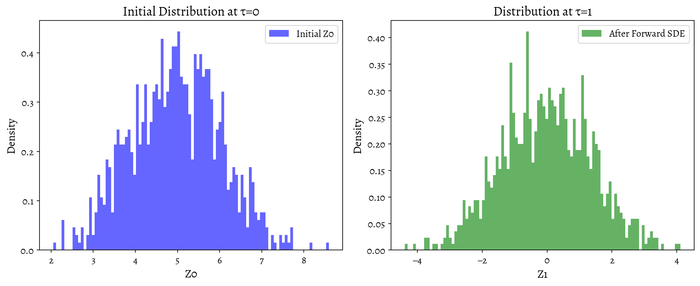
Instead of the stochastic reverse-time SDE, one can use the deterministic probability flow ODE which has the same marginals but no noise term, enabling exact likelihood computation and deterministic sampling (Song et al. 2022).
\[ \boxed{ \frac{dZ_t}{dt} = b(t, Z_t) - \frac{1}{2} a(t) \nabla_z \log p_t(Z_t) } \]
For VE with \(b \equiv 0\) this reduces to \(\frac{dZ_t}{dt} = -\frac{1}{2} a(t) \nabla_z \log p_t(Z_t)\).
This deterministic ODE produces the same marginal distributions \(p_t(z)\) as the reverse-time SDE, but follows a single deterministic trajectory rather than a stochastic one.
4 Fokker-Planck derivation
Now it might not be obvious what \(a\) and \(b\) would produce the desired result in the forward case, let alone how the reverse bit works. It was not to me. There is a traditional explanation that involves saying Fokker-Planck a lot.
4.1 Forward SDE and Density
Suppose the forward SDE is: \[ dZ_{\tau} = b(\tau, Z_{\tau})\,d\tau + \sigma(\tau)\,dW_{\tau}, \quad \tau \in [0,T]. \] Let \(p(t,x)\) be the probability density of \(Z_t\). Then \(p(t,x)\) satisfies the forward Kolmogorov (Fokker-Planck) equation: \[ \partial_t p(t,x) = -\nabla_x \cdot [b(t,x)p(t,x)] + \tfrac{1}{2}\nabla_x \cdot [\sigma(t)\sigma(t)^T \nabla_x p(t,x)]. \]
This equation describes how the density of the process evolves forward in time.
4.2 The Reversed-Time Process and Its Density
Now define the reversed-time process \(\overleftarrow{Z}_\tau := Z_{T-\tau}\) for \(\tau \in [0,T].\) We would like to find an SDE of the form \[ d\overleftarrow{Z}_{\tau} = \overleftarrow{b}(\tau,\overleftarrow{Z}_{\tau})\,d\tau + \sigma(T-\tau)\, d\overleftarrow{W}_{\tau} \] for some drift \(\overleftarrow{b}(\tau,x)\).
The law of \(\overleftarrow{Z}_\tau\) at time \(\tau\) is the same as the law of \(Z_{T-\tau}\). Hence its density at time \(\tau\) should be \(p(T-\tau,x)\).
To summarize: - Forward process \(Z_t\) has density \(p(t,x)\). - Reversed process \(\overleftarrow{Z}_\tau := Z_{T-\tau}\) has density \(\overleftarrow{p}(\tau,x) = p(T-\tau,x)\).
4.3 Forward Equation for the Reversed Density
If \(\overleftarrow{Z}_\tau\) satisfies \[ d\overleftarrow{Z}_{\tau} = \overleftarrow{b}(\tau,x)\,d\tau + \sigma(T-\tau)\,d\overleftarrow{W}_{\tau}, \] then \(\overleftarrow{p}(\tau,x)\) must satisfy its own forward Kolmogorov equation in \(\tau\): \[ \partial_{\tau}\overleftarrow{p}(\tau,x) = -\nabla_x \cdot[\overleftarrow{b}(\tau,x)\overleftarrow{p}(\tau,x)] + \tfrac{1}{2}\nabla_x \cdot[\sigma(T-\tau)\sigma(T-\tau)^T \nabla_x \overleftarrow{p}(\tau,x)]. \]
Since \(\overleftarrow{p}(\tau,x) = p(T-\tau,x)\), we can rewrite this in terms of \(p\): \[ \partial_{\tau} p(T-\tau,x) = -\nabla_x \cdot[\overleftarrow{b}(\tau,x)p(T-\tau,x)] + \tfrac{1}{2}\nabla_x \cdot[\sigma(T-\tau)\sigma(T-\tau)^T \nabla_x p(T-\tau,x)]. \]
4.4 Back to the Original Forward Equation
From the original PDE for \(p(t,x)\), we have: \[ \partial_t p(t,x) = -\nabla_x \cdot[b(t,x)p(t,x)] + \tfrac{1}{2}\nabla_x \cdot[\sigma(t)\sigma(t)^T \nabla_x p(t,x)]. \]
Replace \(t\) by \(T-\tau\): \[ \partial_{T-\tau} p(T-\tau,x) = -\nabla_x \cdot[b(T-\tau,x)p(T-\tau,x)] + \tfrac{1}{2}\nabla_x \cdot[\sigma(T-\tau)\sigma(T-\tau)^T \nabla_x p(T-\tau,x)]. \]
Taking into account that \(\partial_{T-\tau} = -\partial_{\tau}\), we get: \[ -\partial_{\tau} p(T-\tau,x) = -\nabla_x \cdot[b(T-\tau,x)p(T-\tau,x)] + \tfrac{1}{2}\nabla_x \cdot[\sigma(T-\tau)\sigma(T-\tau)^T \nabla_x p(T-\tau,x)]. \]
Multiply through by \(-1\): \[ \partial_{\tau} p(T-\tau,x) = \nabla_x \cdot[b(T-\tau,x)p(T-\tau,x)] - \tfrac{1}{2}\nabla_x \cdot[\sigma(T-\tau)\sigma(T-\tau)^T \nabla_x p(T-\tau,x)]. \]
4.5 Solving the Two PDEs
We have two expressions for \(\partial_{\tau} p(T-\tau,x)\):
From the reversed SDE perspective: \[ \partial_{\tau} p(T-\tau,x) = -\nabla_x \cdot[\overleftarrow{b}(\tau,x)p(T-\tau,x)] + \tfrac{1}{2}\nabla_x \cdot[\sigma(T-\tau)\sigma(T-\tau)^T \nabla_x p(T-\tau,x)]. \]
From the original PDE transformed in time: \[ \partial_{\tau} p(T-\tau,x) = \nabla_x \cdot[b(T-\tau,x)p(T-\tau,x)] - \tfrac{1}{2}\nabla_x \cdot[\sigma(T-\tau)\sigma(T-\tau)^T \nabla_x p(T-\tau,x)]. \]
Set these equal to each other: \[ -\nabla_x \cdot[\overleftarrow{b}(\tau,x)p(T-\tau,x)] + \tfrac{1}{2}\nabla_x \cdot[\sigma(T-\tau)\sigma(T-\tau)^T \nabla_x p(T-\tau,x)] = \nabla_x \cdot[b(T-\tau,x)p(T-\tau,x)] - \tfrac{1}{2}\nabla_x \cdot[\sigma(T-\tau)\sigma(T-\tau)^T \nabla_x p(T-\tau,x)]. \]
Move all terms involving \(\nabla_x p(T-\tau,x)\) together: \[ -\nabla_x \cdot[\overleftarrow{b}(\tau,x)p(T-\tau,x)] = \nabla_x \cdot[b(T-\tau,x)p(T-\tau,x)] - \nabla_x \cdot[\sigma(T-\tau)\sigma(T-\tau)^T \nabla_x p(T-\tau,x)]. \]
4.6 Factor and Divide by the Density
The key step: to isolate \(\overleftarrow{b}\), we divide through by \(p(T-\tau,x)\). Before doing that, we rewrite the equation explicitly. Notice that: \[ \nabla_x \cdot[\overleftarrow{b}(\tau,x)p(T-\tau,x)] = p(T-\tau,x)\nabla_x \cdot \overleftarrow{b}(\tau,x) + \overleftarrow{b}(\tau,x)\cdot \nabla_x p(T-\tau,x). \]
Similarly, \[ \nabla_x \cdot[b(T-\tau,x)p(T-\tau,x)] = p(T-\tau,x)\nabla_x \cdot b(T-\tau,x) + b(T-\tau,x)\cdot \nabla_x p(T-\tau,x). \]
And \[ \nabla_x \cdot[\sigma(T-\tau)\sigma(T-\tau)^T \nabla_x p(T-\tau,x)] = \sigma(T-\tau)\sigma(T-\tau)^T : \nabla_x^2 p(T-\tau,x), \] where “:” denotes the Frobenius inner product. But it’s more intuitive to keep it in divergence form.
Now divide every term by \(p(T-\tau,x)\). This gives us terms like \(\frac{\nabla_x p(T-\tau,x)}{p(T-\tau,x)}\), which is precisely \(\nabla_x \log p(T-\tau,x)\).
After dividing by \(p(T-\tau,x)\), terms organize as follows. We get an equation of the form: \[ - \overleftarrow{b}(\tau,x) - \overleftarrow{b}(\tau,x)\cdot \nabla_x \log p(T-\tau,x) = b(T-\tau,x) + b(T-\tau,x)\cdot \nabla_x \log p(T-\tau,x) - \sigma(T-\tau)\sigma(T-\tau)^T \nabla_x \log p(T-\tau,x). \]
By carefully rearranging (grouping terms involving \(\overleftarrow{b}\), and then isolating \(\overleftarrow{b}\)), one finds the well-known formula: \[ \overleftarrow{b}(\tau,x) = -b(T-\tau,x) + \sigma(T-\tau)\sigma(T-\tau)^T \nabla_x \log p(T-\tau,x). \]
The appearance of the score \(\log p(T-\tau,x)\) is due precisely to this division by \(p(T-\tau,x)\). When we go from equations involving \(p\) to equations involving velocities or drifts that must be expressed in terms of more fundamental gradients, we get the ratio \(\frac{\nabla_x p}{p}\), which is \(\nabla_x \log p\).