Score diffusion

2.1 The Backward SDE and Its Drift Term

The backward SDE is given by:

\[ dZ_{\tau} = \left[ b(\tau) Z_{\tau} - \sigma^2(\tau) S_{\text{posterior}}(Z_{\tau}, \tau) \right] d\tau + \sigma(\tau) d\overleftarrow{W}_{\tau} \]

• \(S_{\text{posterior}}(Z_{\tau}, \tau) = \nabla_z \log q_{Z_{\tau}}(Z_{\tau})\) is the score function of the distribution at time \(\tau\).
• The drift term is \(\mu(z, \tau) = b(\tau) z - \sigma^2(\tau) S_{\text{posterior}}(z, \tau)\).

Our goal is to show that with this drift term, the distribution \(q_{Z_{0}}(z)\) at \(\tau = 0\) is the desired posterior distribution \(p_{X|Y}(x|y)\).

2.2 The Fokker-Planck Equation and Density Evolution

The Fokker-Planck equation describes how the probability density \(q_{Z_{\tau}}(z)\) evolves over time under the influence of the SDE:

\[ \frac{\partial q_{Z_{\tau}}(z)}{\partial \tau} = -\nabla_z \cdot \left[ \mu(z, \tau) q_{Z_{\tau}}(z) \right] + \frac{1}{2} \sigma^2(\tau) \Delta_z q_{Z_{\tau}}(z) \]

• \(\nabla_z \cdot\) denotes the divergence operator.
• \(\Delta_z\) is the Laplacian operator with respect to \(z\).

2.3 Incorporating the Posterior Score Function

The posterior score function can be expressed as:

\[ S_{\text{posterior}}(z, \tau) = S_{\text{prior}}(z, \tau) + h(\tau) \nabla_z \log p_{Y|X}(y | z) \]

• \(S_{\text{prior}}(z, \tau)\) is the prior score function.
• \(h(\tau)\) is a damping function, typically chosen as \(h(\tau) = 1 - \tau\).
• \(\nabla_z \log p_{Y|X}(y | z)\) is the gradient of the log-likelihood.

By setting the drift term using \(S_{\text{posterior}}(z, \tau)\), we adjust the evolution of \(q_{Z_{\tau}}(z)\) to incorporate the influence of the observation \(y\).

2.4 Evolution Towards the Posterior Distribution

At \(\tau = 1\):

• The distribution \(q_{Z_{1}}(z)\) is known (e.g., standard normal distribution).

For \(\tau \in [0, 1]\):

• The backward SDE evolves the distribution \(q_{Z_{\tau}}(z)\) backward in time.
• The drift term includes the posterior score function, guiding the density towards the posterior distribution.

As \(\tau \rightarrow 0\):

• The damping function \(h(\tau) \rightarrow 1\), so the influence of the likelihood becomes fully incorporated.
• The distribution \(q_{Z_{0}}(z)\) approaches the posterior distribution \(p_{X|Y}(x|y)\).

2.5 Mathematical Justification Using the Fokker-Planck Equation

3.1 The Likelihood and Its Gradient

• Likelihood:

  \[ p_{Y|X}(y | x) = \frac{1}{\sqrt{2\pi \sigma^2}} \exp\left( -\frac{(y - \sin(x))^2}{2\sigma^2} \right) \]

• Gradient of Log-Likelihood:

  \[ \nabla_x \log p_{Y|X}(y | x) = \frac{y - \sin(x)}{\sigma^2} \cos(x) \]

3.2 Posterior Score Function

The posterior score function is:

\[ S_{\text{posterior}}(x, \tau) = S_{\text{prior}}(x, \tau) + h(\tau) \frac{y - \sin(x)}{\sigma^2} \cos(x) \]

• As \(\tau \rightarrow 0\), \(h(\tau) \rightarrow 1\), and the influence of the likelihood is fully incorporated.

3.3 Evolution of the Density

By including this posterior score function in the drift term of the backward SDE, we adjust the evolution of \(q_{Z_{\tau}}(z)\) to move towards the posterior distribution \(p_{X|Y}(x|y)\).

• Drift Term in Backward SDE:

  \[ \mu(z, \tau) = b(\tau) z - \sigma^2(\tau) \left( S_{\text{prior}}(z, \tau) + h(\tau) \frac{y - \sin(z)}{\sigma^2} \cos(z) \right) \]

At \(\tau = 0\):

• The evolution governed by the Fokker-Planck equation with the above drift term ensures that \(q_{Z_{0}}(z) = p_{X|Y}(x|y)\).
• This means that the samples \(Z_{0}\) obtained from the backward SDE at \(\tau = 0\) are distributed according to the desired posterior distribution.

4.1 Import Libraries

import jax
import jax.numpy as jnp
import numpy as np
from jax import random, grad
import matplotlib.pyplot as plt
from livingthing.matplotlib_style import set_livingthing_style, reset_default_style

set_livingthing_style()

4.2 Define SDE Coefficients

We set \(\alpha_{\tau} = 1 - \tau\) and \(\beta_{\tau}^2 = \tau\), leading to

def b_tau(tau):
    return -1.0 / (1.0 - tau)

def sigma_tau(tau):
    return jnp.sqrt(1.0 + 2.0 * tau / (1.0 - tau))

4.3 Define the Observation Model and Score Function

Let \(g(x) = \sin(x)\) and assume Gaussian noise \(\varepsilon \sim \mathcal{N}(0, \sigma^2)\). The likelihood is:

\[ p(Y=y|X=x) = \mathcal{N}(y | \sin(x), \sigma^2) \]

Thus, the gradient of the log-likelihood is:

\[ \nabla_x \log p(Y=y|X=x) = \frac{y - \sin(x)}{\sigma^2} \cos(x) \]

Define the score function incorporating the posterior:

def posterior_score(z, tau, y, sigma2):
    # Score of the prior (assuming q(Z_tau) is standard normal for simplicity)
    score_prior = -z / tau  # From S_prior = -z / tau for q(Z_tau) = N(0, tau)

    # Gradient of log-likelihood
    grad_log_likelihood = (y - jnp.sin(z)) / sigma2 * jnp.cos(z)

    # Damping function h(tau) = 1 - tau
    h_tau = 1.0 - tau

    # Posterior score
    return score_prior + h_tau * grad_log_likelihood

4.4 Forward SDE Simulation

Simulate the forward diffusion process, adding noise to the data:

def simulate_forward_sde(Z0, key, N=1000):
    dtau = 1.0 / N
    tau_values = jnp.linspace(0.0, 1.0, N + 1)
    Z_tau = Z0
    Z_tau_list = [Z_tau]

    for i in range(N):
        tau = tau_values[i]
        b = b_tau(tau)
        sigma = sigma_tau(tau)
        key, subkey = random.split(key)
        dW = random.normal(subkey, shape=Z0.shape) * jnp.sqrt(dtau)
        Z_tau = Z_tau + b * Z_tau * dtau + sigma * dW
        Z_tau_list.append(Z_tau)

    return jnp.array(Z_tau_list)

4.5 Backward SDE Simulation

Simulate the backward denoising process, incorporating the posterior score:

def simulate_backward_sde(Z1, y, sigma2, key, N=1000):
    dtau = -1.0 / N  # Negative time step for backward integration
    tau_values = jnp.linspace(1.0, 0.0, N + 1)
    Z_tau = Z1
    Z_tau_list = [Z_tau]

    for i in range(N):
        tau = tau_values[i]
        b = b_tau(tau)
        sigma = sigma_tau(tau)
        S_posterior = posterior_score(Z_tau, tau, y, sigma2)
        drift = b * Z_tau - sigma**2 * S_posterior
        key, subkey = random.split(key)
        dW = random.normal(subkey, shape=Z1.shape) * jnp.sqrt(-dtau)
        Z_tau = Z_tau + drift * dtau + sigma * dW
        Z_tau_list.append(Z_tau)

    return jnp.array(Z_tau_list)

4.6 Example Usage

Simulate both processes with a non-trivial observation model and visualize the results.

# Initialize random keys
key = random.PRNGKey(0)
key, subkey = random.split(key)

# Number of samples and time steps
num_samples = 10000
N = 1000

# Observation parameters
y = 0.5  # Observed value
sigma2 = 0.1  # Variance of observation noise

# Initial data distribution: X ~ N(5, 1)
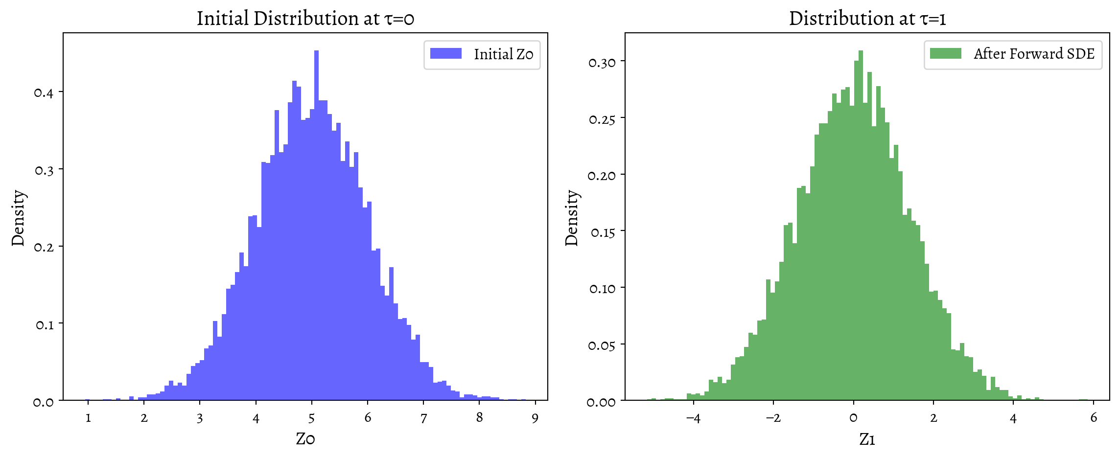
Z0 = random.normal(subkey, shape=(num_samples,)) * 1.0 + 5.0

# Simulate forward SDE
key, subkey = random.split(key)
Z_forward = simulate_forward_sde(Z0, subkey, N=N)

# Simulate backward SDE starting from Z1
Z1 = Z_forward[-1]
key, subkey = random.split(key)
Z_backward = simulate_backward_sde(Z1, y, sigma2, subkey, N=N)

# Convert to numpy for plotting
Z0_np = np.array(Z0)
Z1_np = np.array(Z1)
Z_backward_np = np.array(Z_backward[-1])

# Plotting the distributions
plt.figure(figsize=(18, 5))

# Initial distribution
plt.subplot(1, 3, 1)
plt.hist(Z0_np, bins=100, density=True, alpha=0.6, color='blue', label='Initial Z0')
plt.title('Initial Distribution at τ=0')
plt.xlabel('Z0')
plt.ylabel('Density')
plt.legend()

# After Forward SDE
plt.subplot(1, 3, 2)
plt.hist(Z1_np, bins=100, density=True, alpha=0.6, color='green', label='After Forward SDE')
plt.title('Distribution at τ=1')
plt.xlabel('Z1')
plt.ylabel('Density')
plt.legend()

# # After Backward SDE
# plt.subplot(1, 3, 3)
# plt.hist(Z_backward_np, bins=100, density=True, alpha=0.6, color='red', label='Recovered Z0')
# plt.title('Recovered Distribution at τ=0')
# plt.xlabel('Z0 Recovered')
# plt.ylabel('Density')
# plt.legend()

plt.tight_layout()
plt.show()