Stationary Gamma processes

October 14, 2019 — April 8, 2022

algebra
geometry
linear algebra
Lévy processes
measure
probability
signal processing
sparser than thou
stochastic processes
time series

\[\renewcommand{\var}{\operatorname{Var}} \renewcommand{\corr}{\operatorname{Corr}} \renewcommand{\dd}{\mathrm{d}} \renewcommand{\vv}[1]{\boldsymbol{#1}} \renewcommand{\rv}[1]{\mathsf{#1}} \renewcommand{\vrv}[1]{\vv{\rv{#1}}} \renewcommand{\disteq}{\stackrel{d}{=}} \renewcommand{\gvn}{\mid} \renewcommand{\Ex}{\mathbb{E}} \renewcommand{\Pr}{\mathbb{P}}\]

Processes with Gamma marginals. Usually when we discuss Gamma processes we mean Gamma-Lévy processes. Such processes have independent Gamma increments, much like a Wiener process has independent Gaussian increments and a Poisson process has independent Poisson increments. Gamma processes provide the classic subordinator models, i.e. non-decreasing Lévy processes.

There are other processes with Gamma marginals. Much like the Gaussian process family includes many processes with Gaussian marginals, so does the Gamma. It has a different set of natural algebraic relations to the Gaussian process. For example, the class of Gaussian processes is closed under addition and multiplication. The class of Gamma processes is closed under addition and thinning and some other weirder operations, all of which requires little more background knowledge to understand. It turns out there are complications with multivariate Gamma processes so those are handled separately.

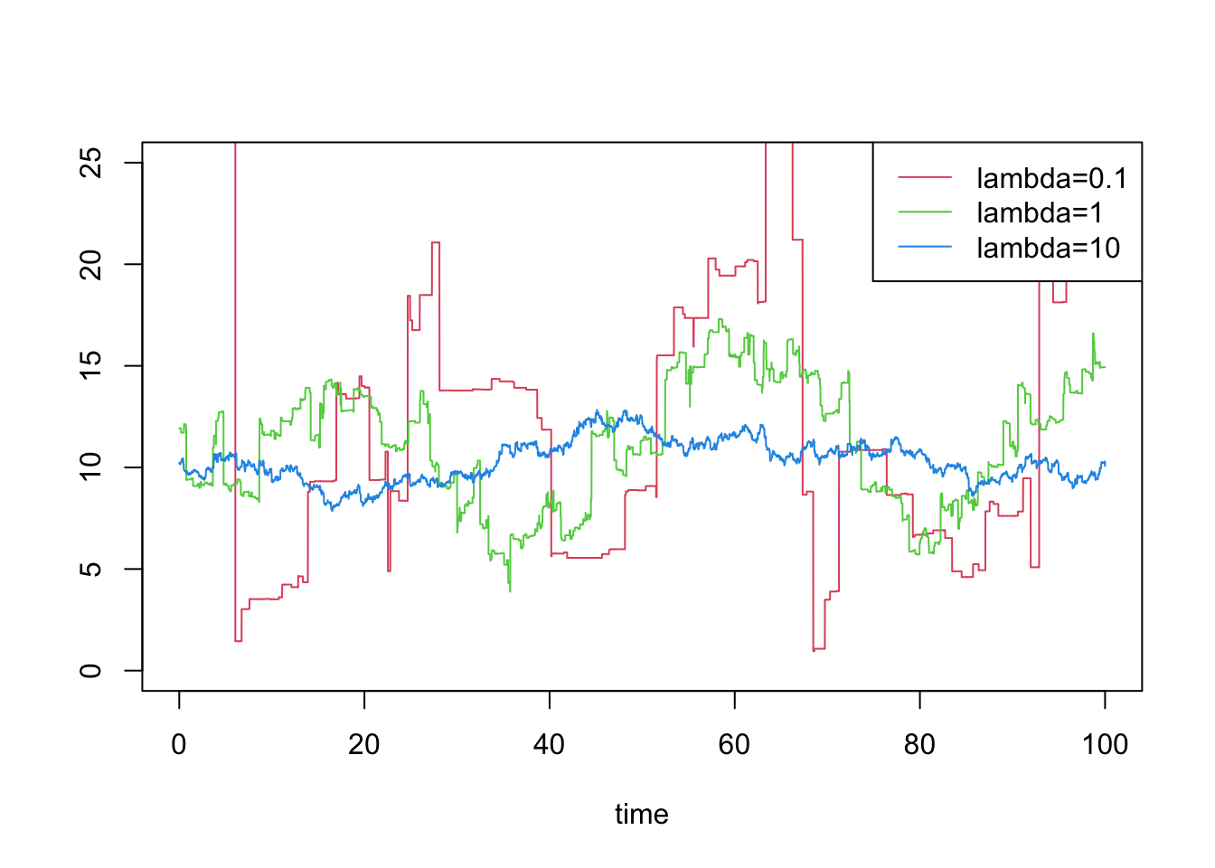
Figure 1: Gamma processes are a natural model for spiky things

Gamma distributions and processes and such crop up all over the place. See also Pólya-Gamma distribution.

OK but if a process’s marginals are “Gamma-distributed”, what does that even mean? First, go and read about Gamma distributions. From that we can construct the Lévy Gamma process which is usually what we mean when we talk about Gamma processes. However, there are many more processes that we can construct with Gamma marginals; those others are here.

THEN go and read about Beta and Dirichlet distributions. and the Gamma-Beta notebook.

Now we are ready to look at stationary dependent Gamma processes.

There are Ornstein–Uhlenbeck-type constructions for Gamma processes (Gaver and Lewis 1980). See R. L. Wolpert (2021) for a modern summary and overview of several popular alternatives.

For fixed \(\alpha, \lambda>0\) these notes present six different stationary time series, each with Gamma \(\rv{g}(t) \sim \operatorname{Gamma}(\alpha, \lambda)\) univariate marginal distributions and autocorrelation function \(\rho^{|s-t|}\) for \(\rv{g}(s), \rv{g}(t)\). Each will be defined on some time index set \(\mathcal{T}\), either \(\mathcal{T}=\mathbb{\rv{z}}\) or \(\mathcal{T}=\mathbb{R}\).

Five of the six constructions can be applied to other Infinitely Divisible (ID) distributions as well, both continuous ones (normal, \(\alpha\)-stable, etc.) and discrete (Poisson, negative binomial, etc). For specifically the Poisson and Gaussian distributions, all but one of them (the Markov change-point construction) coincide — essentially, there is just one “AR(1)-like” Gaussian process (namely, the \(A R(1)\) process in discrete time, or the Ornstein-Uhlenbeck process in continuous time), and there is just one \(A R(1)\)-like Poisson process. For other ID distributions, however, and in particular for the Gamma, each of these constructions yields a process with the same univariate marginal distributions and the same autocorrelation but with different joint distributions at three or more times.

1 Thinned Autoregressive Gamma

To my mind the most natural one.

We let \[ \rv{g}(0) \sim \operatorname{Gamma}(\alpha, \lambda) \] and, for \(t \in \mathbb{N}\) set \[ \rv{g}(t):=\xi(t)+\zeta(t) \] where \[ \begin{aligned} &\xi(t):=\rv{b}(t) \cdot \rv{g}(t-1), \quad \rv{b}(t) \sim \operatorname{Beta}(\alpha \rho, \alpha \bar{\rho}) \\ &\zeta(t) \sim \operatorname{Gamma}(\alpha \bar{\rho}, \lambda) \end{aligned} \] where \(\bar{\rho}:=(1-\rho)\) and all the \(\left\{\rv{b}(t)\right\}\) and \(\left\{\zeta(t)\right\}\) are independent. Then,\(\xi(t) \sim \operatorname{Gamma}(\alpha \rho, \lambda)\) and \(\zeta(t) \sim \operatorname{Gamma}(\alpha \bar{\rho}, \lambda)\) are independent, with sum \(\rv{g}(t) \sim\) \(\operatorname{Gamma}(\alpha, \lambda)\). Thus \(\left\{\rv{g}(t)\right\}\) is a Markov process with Gamma univariate marginal distribution \(\rv{g}(t) \sim \operatorname{Gamma}(\alpha, \lambda)\), now with joint characteristic function \[ \begin{aligned} \chi(s, t) &=\mathbb{E}\exp\left(i s \rv{g}(0)+i t \rv{g}(1)\right) \\ &=\mathbb{E}\exp\left\{i s\left(\rv{g}(0)-\xi(1)\right)+i(s+t) \xi(1)+i t \zeta(1)\right\} \\ &=(1-i s / \lambda)^{-\alpha \bar{\rho}}(1-i(s+t) / \lambda)^{-\alpha \rho}(1-i t / \lambda)^{-\alpha \bar{\rho}} \end{aligned} \] Note that unlike the autoregressive construction, this characteristic function of this one is symmetric in the time arguments, and therefore the process is time-reversible. In some senses this is a “more natural” autoregressive process than the Zeta-innovation AR(1) process. For one, it is easy to imagine how to generalize this to vector autoregressive processes. For another, there is a natural generalization to continuous time (R. L. Wolpert 2021, 2.6) using the Beta process in the sense of Hjort (1990) and Thibaux and Jordan (2007).

What does this look like in practice?

Code
set.seed(105)
# generate a stationary thinned autoregressive Gamma series
gamp = function(T, alpha, lambda, rho) {
  g = rgamma(1, alpha, rate=lambda)
  b = rbeta(T, alpha*rho, alpha*(1-rho))
  zeta = rgamma(T, alpha*(1-rho), rate=lambda)
  gs = numeric(T)
  for (i in 1:T) {
    g = b[i] * g + zeta[i]
    gs[i] = g
  }
  gs
}
T = 10000
ts = (1:T)/100
plot(ts, gamp(T, 1.0, 0.1, 0.999),
    type = "l", col = 2,
    ylim = c(0, 25), ylab="", xlab = "time")
lines(ts, gamp(T, 10, 1.0, 0.999),
    type = "l", col = 3)
lines(ts, gamp(T, 100, 10.0, 0.999),
    type = "l", col = 4)
legend("topright",
       c("lambda=0.1", "lambda=1", "lambda=10"),
       lty = 1, col = 2:4)

2 Additive Zeta innovations

Fix \(0 \leq \rho<1\). Let \(\rv{g}(0) \sim \operatorname{Gamma}(\alpha, \lambda)\) and for \(t \in \mathbb{N}\) define \(\rv{g}(t)\) recursively by \[ \rv{g}(t):=\rho \rv{g}(t-1)+\zeta(t) \] for iid \(\left\{\zeta(t)\right\}\) (see Zeta distribution). The process \(\left\{\rv{g}(t)\right\}\) has Gamma univariate marginal distribution \(\rv{g}(t) \sim \operatorname{Gamma}(\alpha, \lambda)\) for every \(t \in \mathbb{R}_{+}\) and, at consecutive times \(s,t\) joint characteristic function \[ \begin{aligned} \chi(s, t) &=\operatorname{E} \exp \left(i s \rv{g}(0)+i t \rv{g}(1)\right) \\ &=\operatorname{E} \exp \left(i(s+\rho t) \rv{g}(0)+i t \zeta(1)\right) \\ &=\left[\frac{(1-i(s+\rho t) / \lambda)(1-i t / \lambda)}{1-i t \rho / \lambda}\right]^{-\alpha}. \end{aligned} \] Unlike Gaussian additive autoregressive processes, where the marginal and innovation processes are both Gaussian, in Gamma additive autoregressive processes the marginal is Gamma but the innovation is not (Lawrance 1982; Walker 2000). We can get a process that has a gamma innovation by the next construction instead.

Exercise: Generalise this to continuous time.

2.1 Gamma-Zeta distribution

I don’t know a name for the distribution of the \(\zeta(t)\) RVs from earlier. Let us go with Gamma-Zeta, because plain Zeta is taken.

It is easiest to describe that RV in terms of the characteristic function \(E e^{i \omega \zeta(t)}=(1-i \omega / \lambda)^{-\alpha}(1-i \rho \omega / \lambda)^{\alpha}=\left[\frac{\lambda-i \omega}{\lambda-i \rho \omega}\right]^{-\alpha}.\)

Simulating such RVs is easy via the algorithm of Walker (2000):

\[\lambda(t) \sim \operatorname{Gamma}(\alpha, 1), \quad N(t)|\lambda(t) \sim \mathrm{Po}\left(\frac{1-\rho}{\rho} \lambda(t)\right), \quad \zeta(t)| N(t) \sim \operatorname{Gamma}\left(N(t), \frac{\lambda}{\rho}\right).\]

However, this distribution does not seem to have an obvious density except as a Fourier transform. Let us set is aside for now, eh?

3 Change-point gamma

Also from R. L. Wolpert (2021). What other marginals than Gamma can I construct with this?

Let \(\left\{\zeta_{n}: n \in \mathbb{Z}\right\} \stackrel{\text { iid }}{\sim} \mathrm{Ga}(\alpha, \beta)\) be iid Gamma random variables and let \(N_{t}\) be a standard Poisson process indexed by \(t \in \mathbb{R}\) (so \(N_{0}=0\) and \(\left(N_{t}-N_{s}\right) \sim \mathrm{Po}(t-s)\) for all \(-\infty<s<\) \(t<\infty\), with independent increments), and set \[ X_{t}:=\zeta_{n}, \quad n=N_{\lambda t} \] Then each \(X_{t} \sim \mathrm{Ga}(\alpha, \beta)\) and, for \(s, t \in \mathbb{R}, X_{s}\) and \(X_{t}\) are either identical (with probability \(\left.\rho^{|s-t|}\right)\) or independent- reminiscent of a Metropolis MCMC chain. The chf is \[ \begin{aligned} \chi(s, t) &=\mathrm{E} \exp \left(i s X_{0}+i t X_{1}\right) \\ &=\rho(1-i(s+t) / \beta)^{-\alpha}+\bar{\rho}(1-i s / \beta)^{-\alpha}(1-i t / \beta)^{-\alpha} \end{aligned} \] and once again the marginal distribution is \(X_{t} \sim \mathrm{Ga}(\alpha, \beta)\) and the autocorrelation function is \(\operatorname{Corr}\left(X_{s}, X_{t}\right)=\rho^{|s-t|}\).

4 Matrix-valued Gamma-like processes

See matrix and vector Gamma processes.

5 References

Ahrens, and Dieter. 1974. Computer Methods for Sampling from Gamma, Beta, Poisson and Bionomial Distributions.” Computing.
———. 1982. Generating Gamma Variates by a Modified Rejection Technique.” Communications of the ACM.
Applebaum. 2004. Lévy Processes — from Probability to Finance and Quantum Groups.” Notices of the AMS.
———. 2009. Lévy Processes and Stochastic Calculus. Cambridge Studies in Advanced Mathematics 116.
Asmussen, and Glynn. 2007. Stochastic Simulation: Algorithms and Analysis.
Avramidis, L’Ecuyer, and Tremblay. 2003. New Simulation Methodology for Finance: Efficient Simulation of Gamma and Variance-Gamma Processes.” In Proceedings of the 35th Conference on Winter Simulation: Driving Innovation. WSC ’03.
Barndorff-Nielsen, Maejima, and Sato. 2006. Some Classes of Multivariate Infinitely Divisible Distributions Admitting Stochastic Integral Representations.” Bernoulli.
Barndorff-Nielsen, Pedersen, and Sato. 2001. Multivariate Subordination, Self-Decomposability and Stability.” Advances in Applied Probability.
Bertoin. 1996. Lévy Processes. Cambridge Tracts in Mathematics 121.
———. 1999. Subordinators: Examples and Applications.” In Lectures on Probability Theory and Statistics: Ecole d’Eté de Probailités de Saint-Flour XXVII - 1997. Lecture Notes in Mathematics.
———. 2000. Subordinators, Lévy Processes with No Negative Jumps, and Branching Processes.
Bhattacharya, and Waymire. 2009. Stochastic Processes with Applications.
Bondesson. 2012. Generalized Gamma Convolutions and Related Classes of Distributions and Densities. Lecture Notes in Statistics 76.
Buchmann, Kaehler, Maller, et al. 2015. Multivariate Subordination Using Generalised Gamma Convolutions with Applications to V.G. Processes and Option Pricing.” arXiv:1502.03901 [Math, q-Fin].
Chaumont, and Yor. 2012. Exercises in Probability: A Guided Tour from Measure Theory to Random Processes, Via Conditioning.
Çinlar. 1980. On a Generalization of Gamma Processes.” Journal of Applied Probability.
Connor, and Mosimann. 1969. “Concepts of Independence for Proportions with a Generalization of the Dirichlet Distribution.” Journal of the American Statistical Association.
Devroye. 1986. Non-uniform random variate generation.
Dufresne. 1998. Algebraic Properties of Beta and Gamma Distributions, and Applications.” Advances in Applied Mathematics.
Edwards, Meyer, and Christensen. 2019. Bayesian Nonparametric Spectral Density Estimation Using B-Spline Priors.” Statistics and Computing.
Émery, and Yor. 2004. A Parallel Between Brownian Bridges and Gamma Bridges.” Publications of the Research Institute for Mathematical Sciences.
Ferguson. 1974. Prior Distributions on Spaces of Probability Measures.” The Annals of Statistics.
Ferguson, and Klass. 1972. A Representation of Independent Increment Processes Without Gaussian Components.” The Annals of Mathematical Statistics.
Figueroa-López. 2012. Jump-Diffusion Models Driven by Lévy Processes.” In Handbook of Computational Finance.
Fink. 1997. A Compendium of Conjugate Priors.”
Foti, Futoma, Rockmore, et al. 2013. A Unifying Representation for a Class of Dependent Random Measures.” In Artificial Intelligence and Statistics.
Gaver, and Lewis. 1980. First-Order Autoregressive Gamma Sequences and Point Processes.” Advances in Applied Probability.
Gourieroux, and Jasiak. 2006. Autoregressive Gamma Processes.” Journal of Forecasting.
Griffiths, and Ghahramani. 2011. The Indian Buffet Process: An Introduction and Review.” Journal of Machine Learning Research.
Grigelionis. 2013. Student’s t-Distribution and Related Stochastic Processes. SpringerBriefs in Statistics.
Grunwald, G K, Hyndman, and Tedesco. 1996. “A Unified View of Linear AR(1) Models.”
Grunwald, Gary K., Hyndman, Tedesco, et al. 2000. Theory & Methods: Non-Gaussian Conditional Linear AR(1) Models.” Australian & New Zealand Journal of Statistics.
Gupta, and Nadarajah, eds. 2014. Handbook of Beta Distribution and Its Applications.
Gusak, Kukush, Kulik, et al. 2010. Theory of Stochastic Processes : With Applications to Financial Mathematics and Risk Theory. Problem Books in Mathematics.
Hackmann, and Kuznetsov. 2016. Approximating Lévy Processes with Completely Monotone Jumps.” The Annals of Applied Probability.
Hjort. 1990. Nonparametric Bayes Estimators Based on Beta Processes in Models for Life History Data.” The Annals of Statistics.
Ishwaran, and Zarepour. 2002. Exact and Approximate Sum Representations for the Dirichlet Process.” Canadian Journal of Statistics.
James, Roynette, and Yor. 2008. Generalized Gamma Convolutions, Dirichlet Means, Thorin Measures, with Explicit Examples.” Probability Surveys.
Kingman. 1992. Poisson Processes.
Kirch, Edwards, Meier, et al. 2019. Beyond Whittle: Nonparametric Correction of a Parametric Likelihood with a Focus on Bayesian Time Series Analysis.” Bayesian Analysis.
Kyprianou. 2014. Fluctuations of Lévy Processes with Applications: Introductory Lectures. Universitext.
Lalley. 2007. “Lévy Processes, Stable Processes, and Subordinators.”
Lawrance. 1982. The Innovation Distribution of a Gamma Distributed Autoregressive Process.” Scandinavian Journal of Statistics.
Lawrence, and Urtasun. 2009. Non-Linear Matrix Factorization with Gaussian Processes.” In Proceedings of the 26th Annual International Conference on Machine Learning. ICML ’09.
Lefebvre. 2007. Applied Stochastic Processes. Universitext.
Lin. 2016. “On The Dirichlet Distribution.”
Liou, Su, Chiang, et al. 2011. Gamma Random Field Simulation by a Covariance Matrix Transformation Method.” Stochastic Environmental Research and Risk Assessment.
Lo, and Weng. 1989. On a Class of Bayesian Nonparametric Estimates: II. Hazard Rate Estimates.” Annals of the Institute of Statistical Mathematics.
Mathai. 1982. Storage Capacity of a Dam with Gamma Type Inputs.” Annals of the Institute of Statistical Mathematics.
Mathai, and Moschopoulos. 1991. On a Multivariate Gamma.” Journal of Multivariate Analysis.
Mathai, and Provost. 2005. Some Complex Matrix-Variate Statistical Distributions on Rectangular Matrices.” Linear Algebra and Its Applications, Tenth Special Issue (Part 2) on Linear Algebra and Statistics,.
Mathal, and Moschopoulos. 1992. A Form of Multivariate Gamma Distribution.” Annals of the Institute of Statistical Mathematics.
Meier. 2018. A matrix Gamma process and applications to Bayesian analysis of multivariate time series.”
Meier, Kirch, Edwards, et al. 2019. beyondWhittle: Bayesian Spectral Inference for Stationary Time Series.”
Meier, Kirch, and Meyer. 2020. Bayesian Nonparametric Analysis of Multivariate Time Series: A Matrix Gamma Process Approach.” Journal of Multivariate Analysis.
Moschopoulos. 1985. The Distribution of the Sum of Independent Gamma Random Variables.” Annals of the Institute of Statistical Mathematics.
Olofsson. 2005. Probability, Statistics, and Stochastic Processes.
Pérez-Abreu, and Stelzer. 2014. Infinitely Divisible Multivariate and Matrix Gamma Distributions.” Journal of Multivariate Analysis.
Pfaffel. 2012. Wishart Processes.” arXiv:1201.3256 [Math].
Polson, Scott, and Windle. 2013. Bayesian Inference for Logistic Models Using Pólya–Gamma Latent Variables.” Journal of the American Statistical Association.
Rao, and Teh. 2009. “Spatial Normalized Gamma Processes.” In Proceedings of the 22nd International Conference on Neural Information Processing Systems. NIPS’09.
Roychowdhury, and Kulis. 2015. Gamma Processes, Stick-Breaking, and Variational Inference.” In Artificial Intelligence and Statistics.
Rubinstein, and Kroese. 2016. Simulation and the Monte Carlo Method. Wiley series in probability and statistics.
Sato. 1999. Lévy Processes and Infinitely Divisible Distributions.
Semeraro. 2008. A Multivariate Variance Gamma Model for Financial Applications.” International Journal of Theoretical and Applied Finance.
Shah, Wilson, and Ghahramani. 2014. Student-t Processes as Alternatives to Gaussian Processes.” In Artificial Intelligence and Statistics.
Shaked, and Shanthikumar. 1988. On the First-Passage Times of Pure Jump Processes.” Journal of Applied Probability.
Sim. 1990. First-Order Autoregressive Models for Gamma and Exponential Processes.” Journal of Applied Probability.
Singpurwalla, Nozer. 1997. Gamma Processes and Their Generalizations: An Overview.” In Engineering Probabilistic Design and Maintenance for Flood Protection.
Singpurwalla, Nozer D., and Youngren. 1993. Multivariate Distributions Induced by Dynamic Environments.” Scandinavian Journal of Statistics.
Steutel, and van Harn. 2003. Infinite Divisibility of Probability Distributions on the Real Line.
Tankov, and Voltchkova. n.d. “Jump-Diffusion Models: A Practitioner’s Guide.”
Thibaux, and Jordan. 2007. Hierarchical Beta Processes and the Indian Buffet Process.” In Proceedings of the Eleventh International Conference on Artificial Intelligence and Statistics.
Thorin. 1977a. On the Infinite Divisbility of the Pareto Distribution.” Scandinavian Actuarial Journal.
———. 1977b. On the Infinite Divisibility of the Lognormal Distribution.” Scandinavian Actuarial Journal.
Tracey, and Wolpert. 2018. Upgrading from Gaussian Processes to Student’s-T Processes.” 2018 AIAA Non-Deterministic Approaches Conference.
van der Weide. 1997. Gamma Processes.” In Engineering Probabilistic Design and Maintenance for Flood Protection.
Veillette, and Taqqu. 2010a. Using Differential Equations to Obtain Joint Moments of First-Passage Times of Increasing Lévy Processes.” Statistics & Probability Letters.
———. 2010b. Numerical Computation of First-Passage Times of Increasing Lévy Processes.” Methodology and Computing in Applied Probability.
Walker. 2000. A Note on the Innovation Distribution of a Gamma Distributed Autoregressive Process.” Scandinavian Journal of Statistics.
Wilson, and Ghahramani. 2011. Generalised Wishart Processes.” In Proceedings of the Twenty-Seventh Conference on Uncertainty in Artificial Intelligence. UAI’11.
Wolpert, Robert L. 2021. Lecture Notes on Stationary Gamma Processes.” arXiv:2106.00087 [Math].
Wolpert, Robert L., and Brown. 2021. Markov Infinitely-Divisible Stationary Time-Reversible Integer-Valued Processes.” arXiv:2105.14591 [Math].
Wolpert, R., and Ickstadt. 1998. Poisson/Gamma Random Field Models for Spatial Statistics.” Biometrika.
Xuan, Lu, Zhang, et al. 2015. Nonparametric Relational Topic Models Through Dependent Gamma Processes.” arXiv:1503.08542 [Cs, Stat].
Yor. 2007. Some Remarkable Properties of Gamma Processes.” In Advances in Mathematical Finance. Applied and Numerical Harmonic Analysis.