Combining kernels
2019-09-16 — 2023-05-01
Wherein Kernels Are Treated as Gaussian-Process Covariance Functions, and It Is Shown That Sums, Products and Warping Are Preserved as Kernels, With Induced Feature Maps Concatenated Rather Than Summed.
A sum or product (or outer sum, or tensor product) of Mercer kernels is still a kernel. For other operations YMMV; let us look at some.
Since talking about kernels in the abstract is confusing, I like to consider a (slightly) more concrete mental model: Which kernels are valid covariance functions for a Gaussian process? This turns out to be a useful way to think about it because it suggests some ways to combine kernels.
1 Operations preserving positivity
For example, in the case of Gaussian processes, suppose that, independently,
\[\begin{aligned} f_{1} &\sim \mathcal{GP}\left(\mu_{1}, k_{1}\right)\\ f_{2} &\sim \mathcal{GP}\left(\mu_{2}, k_{2}\right) \end{aligned}\] then \[ f_{1}+f_{2} \sim \mathcal{GP} \left(\mu_{1}+\mu_{2}, k_{1}+k_{2}\right) \] so \(k_{1}+k_{2}\) is also a kernel.
More generally, if \(k_{1}\) and \(k_{2}\) are two kernels, and \(c_{1}\) and \(c_{2}\) are two positive real numbers, then \[ K(x, x')=c_{1} k_{1}(x, x')+c_{2} k_{2}(x, x') \] is again a kernel. With multiplication as well, we note that all polynomials of kernels where the coefficients are positive are in turn kernels (Genton 2001).
Note that the additivity in terms of kernels is not the same as additivity in terms of induced feature spaces. The induced feature map of \(k_{1}+k_{2}\) is their concatenation rather than their sum. Suppose \(\phi_{1}(x)\) gives us the feature map of \(k_{1}\) for \(x\) and likewise \(\phi_{2}(x)\). Then \[\begin{aligned} k_{1}(x, x') &=\phi_{1}(x)^{\top} \phi_{1}(x') \\ k_{2}(x, x') &=\phi_{2}(x)^{\top} \phi_{2}(x')\\ k_{1}(x, x')+k_{2}(x, x') &=\phi_{1}(x)^{\top} \phi_{1}(x')+\phi_{2}(x)^{\top} \phi_{2}(x')\\ &=\left[\begin{array}{c}{\phi_{1}(x)} \\ {\phi_{2}(x)}\end{array}\right]^{\top} \left[\begin{array}{c}{\phi_{1}(x')} \\ {\phi_{2}(x')}\end{array}\right] \end{aligned}\]
If \(k:\mathcal{Y}\times\mathcal{Y}\to\mathbb{R}\) is a kernel and \(\psi: \mathcal{X}\to\mathcal{Y}\) this is also a kernel
\[\begin{aligned} k_{\psi}:&\mathcal{X}\times\mathcal{X}\to\mathbb{R}\\ & (x,x')\mapsto k_{y}(\psi(x), \psi(x')) \end{aligned}\]
which apparently is now called a deep kernel. If \(k\) is stationary and \(\psi\) is invertible then this is a stationary reducible kernel.
Also if \(A\) is a positive definite operator, then of course it defines a kernel \(k_A(x,x'):=x^{\top}Ax'\)
Genton (2001) uses the interpretation as covariance to construct some other useful combinations.
Let \(h:\mathcal{X}\to\mathbb{R}^{+}\) have a minimum at 0. Then, using the identity for RVs \[ \mathop{\textrm{Cov}}\left(Y_{1}, Y_{2}\right)=\left[\mathop{\textrm{Var}}\left(Y_{1}+Y_{2}\right)-\mathop{\textrm{Var}}\left(Y_{1}-Y_{2}\right)\right] / 4 \]
we find that the following is a kernel
\[ K(x, x')=\frac{1}{4}[h(x+x')-h(x-x')] \]
All these to various cunning combination strategies, which I may return to discuss. 🚧TODO🚧 Some of them are in the references. For example Duvenaud et al. (2013) position their work in the wider field:
There is a large body of work attempting to construct a rich kernel through a weighted sum of base kernels (e.g. Bach 2008; Christoudias, Urtasun, and Darrell 2009). While these approaches find the optimal solution in polynomial time, speed comes at a cost: the component kernels, as well as their hyperparameters, must be specified in advance […]
Hinton and Salakhutdinov (2008) use a deep neural network to learn an embedding; this is a flexible approach to kernel learning but relies upon finding structure in the input density, \(p(x)\). Instead we focus on domains where most of the interesting structure is in \(f(x)\).
Wilson and Adams (2013) derive kernels of the form $ (x − x_0 $), forming a basis for stationary kernels. These kernels share similarities with \(\operatorname{SE} \times \operatorname{Per}\) but can express negative prior correlation, and could usefully be included in our grammar.
See Grosse et al. (2012) for a mind-melting compositional matrix factorisation diagram, constructing a search over hierarchical kernel decompositions.
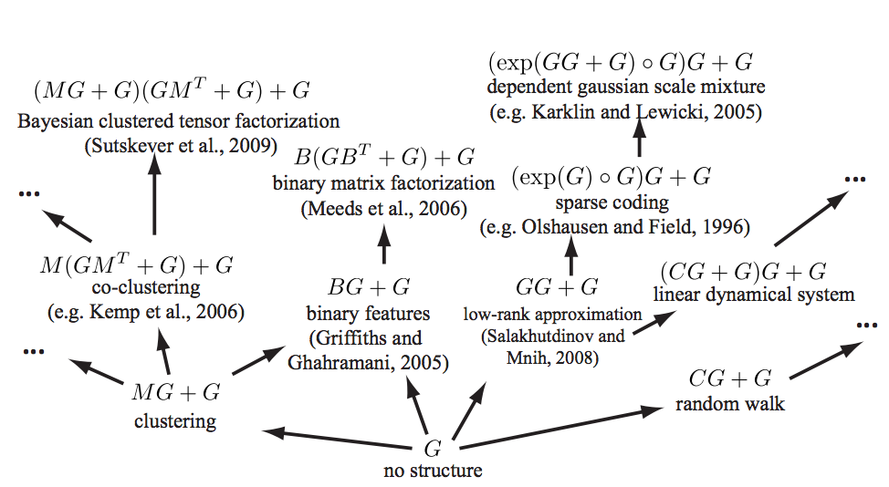
Examples of existing machine learning models which fall under our framework. Arrows represent models reachable using a single production rule. Only a small fraction of the 2496 models reachable within 3 steps are shown, and not all possible arrows are shown.
Here is another list of kernel combinations that preserve positive-definiteness, but for which I have tragically lost the source (it is one of the papers here).
\[ \begin{aligned} K(x, y) &=K_{1}(x, y)+K_{2}(x, y) \\ K(x, y) &=c K_{1}(x, y)+K_{2}(x, y) \text { for } c \in \mathbb{R}_{+} \\ K(x, y) &=K(x, y)+c \text { for } c \in \mathbb{R}_{+} \\ K(x, y) &=K_{1}(x, y) K_{2}(x, y) \\ K(x, y) &=f(x) f(y) \text { for } f: \mathcal{X} \to \mathbb{R} \\ K(x, y) &=\left(K_{1}(x, y)+c\right)^{d} \text { for } c \in \mathbb{R}_{+} \text {and } d \in \mathbb{N} \\ K(x, y) &=\exp \left(K_{1}(x, y) / \sigma^{2}\right) \text { for } \sigma \in \mathbb{R} \\ K(x, y) &=\exp \left(-\left(K(x, x)-2 K(x, y)+K(y, y)\right) / 2 \sigma^{2}\right) \\ K(x, y) &=K_{1}(x, y) / \sqrt{K_{1}(x, x) K_{1}(y, y)} \end{aligned} \]
2 Applying kernels over different axes
I silently assumed this works because it seems obvious sometimes; but then sometimes I forget this trick, so maybe it is not obvious:
For multi-dimensional inputs we can apply kernels over any subset of the axes, and thence different kernels over different subsets of the axes.
3 Locally stationary kernels
Genton (2001) defines locally stationary kernels to mean those that have a particular structure, specifically, a kernel that can be factored into a stationary kernel \(K_2\) and a non-negative function \(K_1\) in the following way:
\[ K(\mathbf{s}, \mathbf{t})=K_{1}\left(\frac{\mathbf{s}+\mathbf{t}}{2}\right) K_{2}(\mathbf{s}-\mathbf{t}) \]
Local structure then depends on the global mean location \(\frac{\mathbf{s}+\mathbf{t}}{2}\). See the paper for some useful spectral properties of these kernels.
Other constructions might vie for the title of “locally stationary”. To check. 🚧TODO🚧
4 Stationary reducible kernels
See kernel warping.