Nearly sufficient statistics and information bottlenecks
Also, rate distortion by other means, and the measure-valued sufficient statistic
2018-03-13 — 2026-05-26
In Which the Posterior Distribution Is Recognised as the Canonical Measure-Valued Sufficient Statistic, Found to Recur Under Many Names Across Disparate Fields, and Subjected to Compression via the Information Bottleneck.
🚧TODO🚧
I’m working through a small realization, for my own interest, which has helped my understanding of variational Bayes; and specifically in relating it to non-Bayes variational inference. Also sequential Monte Carlo.
Finite-dimensional sufficient statistics are the Garden of Edenference. Most problems have no finite-dimensional sufficient statistic, which is to say, their most compact representation is a copy of the prior plus whatever data we’ve seen so far. Or, equivalently, the measure-valued object which is the posterior distribution. Either way, it is a copy of everything we have seen so far.
It seems we manage to act in the world without remembering every experience, however trivial; so if we are doing something like statistical analysis of the world when we learn to act in it, we must be doing so approximately. The question is how cheaply we can approximate that unattainable sufficient statistic measure while losing as little as we can afford to (whatever that, in context, means). Here are some ideas about that.
1 The information bottleneck
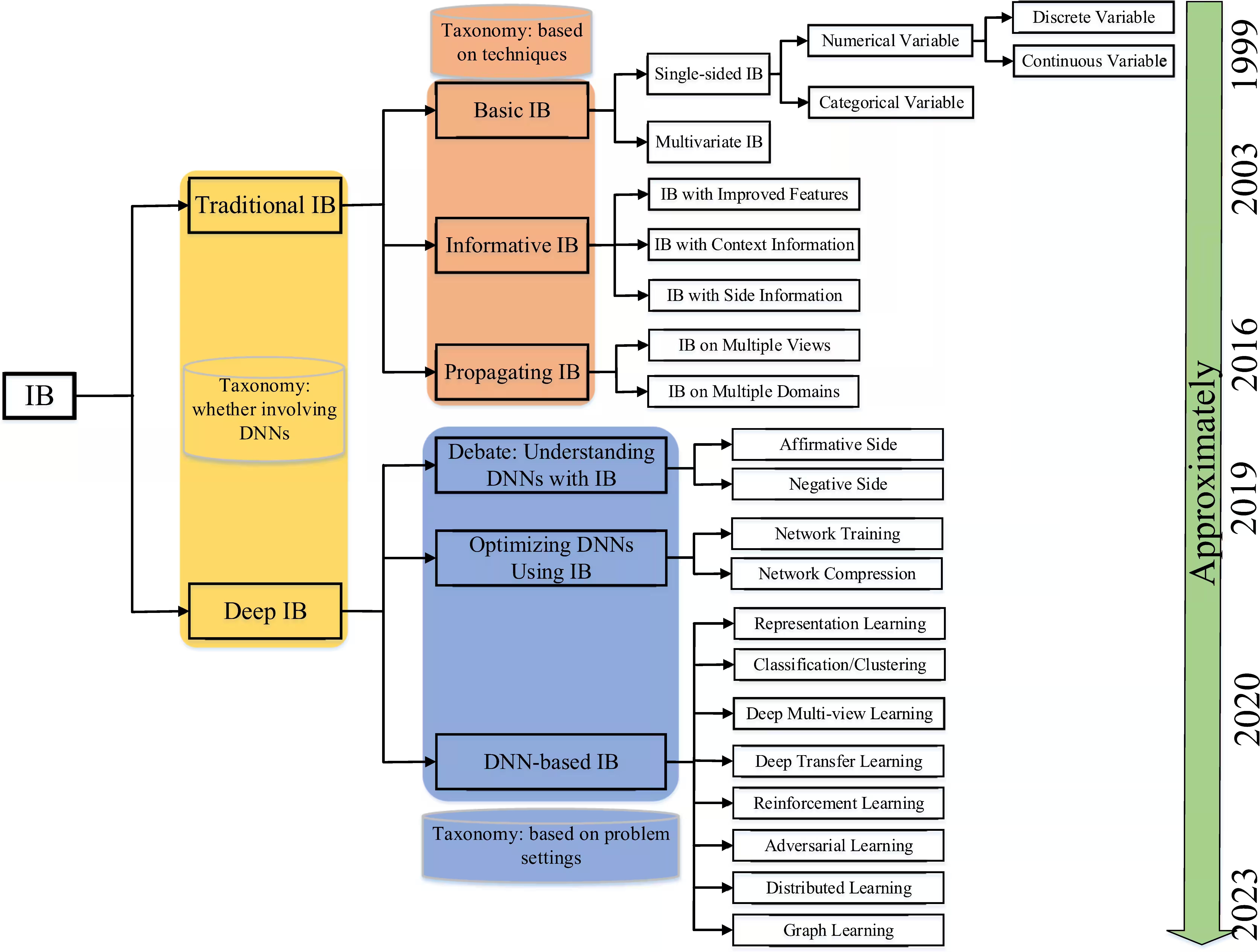
Information bottlenecks are one way of formalising this finite-budget summary of a measure-valued sufficient statistic. I ransacked S. Hu et al. (2024) for a recent summary of developments in information bottleneck theory. Unless otherwise stated, the notation and results come from there.
We pick a “relevance” variable \(Y\) that encodes what matters—future observations, labels, a function of \(\theta\), a decision, or the next state in a filter. Then we find a (hopefully compact) representation \(T\) of \(X\) that trades off compressing \(X\) against preserving information about \(Y\):
\[ \min_{p(t\mid x)}\; I(T;X)\;-\;\beta\, I(T;Y). \]
This is a specialization of rate–distortion, where the distortion is chosen to be the Kullback–Leibler mismatch in predicting \(Y\) from \(T\), and \(\beta\!\!>\!0\) is our trade‑off knob, i.e. rate–distortion with an informational metric.
Payoffs:
- If we set \(Y=\theta\) (or a function of it), the optimal \(T\) is an approximately minimal sufficient statistic for inference about \(\theta\).
- If we set \(Y=X_{t+1}\) (or a future payoff) in a filtering/control problem, we get a predictive state: a compressed memory \(T_t\) of the past that’s maximally useful for predicting what we need next.
1.1 “Nearly sufficient” IB
There are at least two ways to be “nearly sufficient” in the IB context, depending on what we want \(Y\) to do.
Information sufficiency (task‑conditional independence). Define \(T\) to be \(Y\)-sufficient if \(I(Y;X\mid T)=0\). Then “\(\varepsilon\)-sufficient” means \(I(Y;X\mid T)\le \varepsilon\). IB is the convex relaxation that searches for \(T\) with small \(I(T;X)\) subject to small \(I(Y;X\mid T)\), via a Lagrange multiplier \(\beta\).
Decision sufficiency. For a loss \(\ell(a,y)\), call \(T\) \(\varepsilon\)-sufficient if the Bayes risk gap using \(T\) instead of \(X\) is \(\le \varepsilon\). For log‑loss this is equivalent to #1; for other losses it’s stricter or looser. (This is where rate–distortion with a bespoke distortion can be a better fit than vanilla IB if the task isn’t log‑loss‑like.)
Pick the notion that matches our downstream risk. If we’re doing Bayesian filtering or SMC, #1 with \(Y\!=\!X_{t+1}\) or \(Y\!=\!\) future rewards is what we want. On the other hand, if we’re doing parameter estimation, #1 with \(Y\!=\!\theta\) (or a function like \(g(\theta)\)) is usually the cleanest.
1.2 Connection to Variational Bayes
The “deep variational IB” (DVIB) parametrises \(p(t\mid x)\) (the encoder) and works with a variational decoder \(q(y\mid t)\) plus a prior \(r(t)\). The training objective
\[ \max\; \mathbb{E}_{p(t\mid x)}[\log q(y\mid t)]\;-\;\beta\,\mathrm{KL}\big(p(t\mid x)\,\Vert\, r(t)\big) \]
Here’s the IB Lagrangian rewritten so we can optimize it with gradients. With \(Y=X\) and \(\beta\!=\!1\), we recover the VAE ELBO; that’s not an accident. ELBO can be seen as an IB objective where the “relevant” variable is the input itself; DVIB is ELBO with the relevance set to our task.
1.3 Filtering and state compression
In Bayes filtering we want a recursively updated \(T_t\) that is small but “task‑sufficient”. In exponential families (e.g. linear-Gaussian) filters exist, e.g. the Kalman filter.
IB gives us a target for awkward models: minimize \(I(T_t; X_{1:t})\) while maximising \(I(T_t; Y_t)\), where \(Y_t\) is whatever we care about next (the next observation, the latent state, the next reward). We can then:
- Parameter‑tracking: We set \(Y_t=\theta\) (or \(g(\theta)\)), turning \(T_t\) into a rolling compressed posterior proxy.
- Predictive control: We can set \(Y_t=X_{t+1}\) or a function of \(X_{t+1}\) and action \(A_t\).
1.4 In neural nets
Each layer in a trained DNN behaves approximately like a nearly sufficient statistic for its task variable, which is a helpful mental picture even if we don’t care about DNNs. The classical IB principle was defined as an optimization problem over encoders \(p(t|x)\): compress \(X\) into \(T\) while keeping as much information about \(Y\) as possible,
\[ \min_{p(t|x)} I(T;X) - \beta I(T;Y). \]
That’s cool, but impractical as written because neural networks are large and complicated. Deep Information Bottleneck parameterizes the encoder and decoder with neural nets and trains them using gradient methods.
- Encoder: \(p_\theta(t|x)\) (often Gaussian; mean and variance predicted by a neural net).
- Decoder: \(q_\phi(y|t)\), a variational approximation to \(p(y|t)\).
- Prior: \(r(t)\), usually standard Gaussian, to make the KL term computable.
So the training objective becomes:
\[ \max_{\theta,\phi}\; \mathbb{E}_{p_\theta(t|x)}[\log q_\phi(y|t)] - \beta\, \text{KL}(p_\theta(t|x)\|r(t)). \]
That’s the Deep Variational IB (DVIB) objective. If we set \(Y=X\), we get the VAE ELBO; if we set \(Y\) to be labels, we get a bottleneck tuned for classification.
The KL penalty is the mechanism of “compression”. It forces the encoder not to keep every pixel of \(X\) but only the degrees of freedom that actually help predict \(Y\).
This gives the encoder a concrete way to approximate minimal sufficient statistics for \(Y\), even in messy, high-dimensional settings.
Shwartz-Ziv and Tishby (2017) famously plotted layer-wise mutual information during NN training 🚧TODO🚧: I forget now if they were using IB-aware training, or if this holds generally. In their experiments each hidden layer \(T_i\) follows a path in the “information plane” \((I(T;X), I(T;Y))\):
- Phase 1 (fitting): mutual information with \(Y\) shoots up as the layers learn to predict.
- Phase 2 (compression): \(I(T;X)\) falls slowly — the representation forgets irrelevant details while keeping \(I(T;Y)\) high.
The two phases correspond to what we see if we measure gradient statistics: a drift phase (large, directed updates) followed by a diffusion phase (random fluctuations dominate). The diffusion adds noise that automatically compresses representations.
I think this means that in the Deep IB view, SGD itself is a bottleneck machine.* Layers end up very close to the IB theoretical bound, which characterises optimal trade-offs between memory \(I(T;X)\) and relevance \(I(T;Y)\).
1.5 Non-convexity
There are two competing terms in the functional
\[ \min_{p(t|x)} I(T;X) - \beta I(T;Y). \]
\(I(T;X)\) is convex in \(p(t|x)\), while \(I(T;Y)\) is concave in \(p(t|x)\). Their weighted difference is not convex. This means we don’t get the nice guarantees we’d have in rate–distortion theory with convex distortion measures. Instead, the IB Lagrangian can have multiple local minima.
The iterative IB algorithm (the original Blahut–Arimoto-style update rules from Tishby et al. 1999) only converges to a fixed point of the self-consistent equations, not necessarily the global optimum. This is why different runs with different initialisations can produce different clusterings or partitions of the data.
- Classical IB (discrete case): iterative IB converges to locally optimal solutions; sometimes multiple solutions lie on the same “information curve,” but we don’t know if we’ve found the best.
- Deep IB (DVIB): we’ve compounded the problem: now the encoder/decoder are parameterized by neural nets, so we inherit both the non-convexity of the IB objective and the non-convexity of deep learning. Optimizers (SGD, Adam) will tend to settle in some basin that’s “good enough” but not provably optimal.
- Information-plane diagnostics (Schwartz-Ziv & Tishby): One of the reasons they use mutual information plots is to check whether the layers land near the theoretical IB bound. But the fact that different training runs converge to slightly different places reflects the non-convexity.
Researchers have tried to tame this in several ways:
Convex relaxations / surrogates: Variants like the Hilbert–Schmidt independence criterion bottleneck (HSIC-IB) replace mutual information with a kernel-based dependence measure, which yields a convex or easier objective for optimization.
Variational bounds: DVIB itself is a relaxation — we replace intractable mutual information terms with variational lower bounds. These are optimizable with SGD, but they don’t restore convexity; they just make the problem numerically tractable.
Deficiency and f-divergence bottlenecks: Alternatives like the variational deficiency bottleneck (VDB) swap in divergences with better optimization landscapes in some cases.
Annealing β / continuation: A common heuristic is to slowly increase \(\beta\), following the IB curve and avoiding bad local minima.
2 Other nearly-sufficient statistics approaches
Rate–Distortion (RD). Classic source coding. We choose a distortion \(d\) and find the minimal rate \(R(D)\). When our “task” is truly captured by a metric on \(x\)–\(t\) pairs, RD is the cleanest. IB is RD with a data‑driven distortion that says: “Two inputs are close if they induce similar posteriors over \(Y\).”
Coresets / inducing sets. These reduce dataset size rather than feature dimension: we keep a small weighted subset that approximates the full objective. Great for bounded memory and streaming, orthogonal to the IB trade‑off — we can do IB on top of a coreset. See data summarization
MDL (Minimum Description Length). Another compression‑flavoured philosophy. MDL trades codelength of model plus residuals; IB trades mutual information for a chosen relevance. It’s related to Kolmogorov complexity.
3 Also singular learning theory
See Singular learning theory for an implicit approach to “nearly sufficient” statistics, which is more focused on the geometry of the likelihood function and the behaviour of the marginal likelihood in singular models. This comes out rather different for unclear reason.