Ablation studies, knockout studies, lesion studies

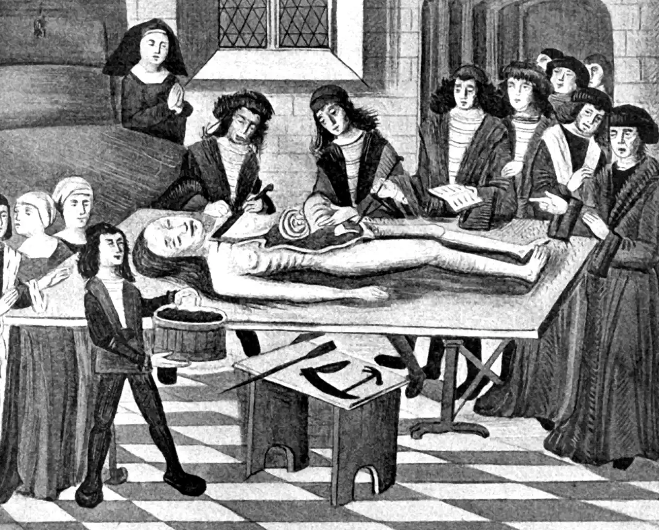
Can we work out how a complex or adaptive system works by destroying bits of it?

This comes up often in the study of complicated things, because there are too many variables, and too many ethical constraints, to do all the experiments we might imagine.

In various fields, it has been asked how far we can push the simple experiment of working out what breaks, which is called an ablation study in neural nets, a lesion study in neuroscience, and a knockout study in genetics.

Questions about the limits of this methodology arise in Can a biologist fix a radio (Lazebnik 2002)? Could a neuroscientist understand a microprocessor (Jonas and Kording 2017)? Should an alien doctor stop human bleeding by removing blood?

The answer, I claim, is it depends. These are classic identifiability from observational data problems. For a methodology which attempts to identify causal structures in a principled fashion, see causal abstraction.

Here is a spicy take which argues that the current state of the model is only understandable in the context of its training history: Interpretability Creationism:

[…] Stochastic Gradient Descent is not literally biological evolution, but post-hoc analysis in machine learning has a lot in common with scientific approaches in biology, and likewise often requires an understanding of the origin of model behaviour. Therefore, the following holds whether looking at parasitic brooding behaviour or at the inner representations of a neural network: if we do not consider how a system develops, it is difficult to distinguish a pleasing story from a useful analysis. In this piece, I will discuss the tendency towards “interpretability creationism” — interpretability methods that only look at the final state of the model and ignore its evolution over the course of training — and propose a focus on the training process to supplement interpretability research.

That essay clearly connects to model explanation, and I think, observational studies generally. If we take that seriously, we might start thinking about developmental interpretability.