Ensemble Kalman updates are empirical Matheron updates

1 Set‑up

Let \(x\in\mathbb R^d\) denote the latent state with prior \(x\sim\mathcal N(m,\Sigma)\), and let \(y=Hx+\varepsilon\) denote the observation with \(\varepsilon\sim\mathcal N(0,R)\). Classical Gaussian conditioning gives:

\[ \begin{aligned} K &= \Sigma H^\top\,(H\Sigma H^\top + R)^{-1},\\ x\mid (y=y^*) &\sim \mathcal N\Bigl(m + K(y^*-Hm),\;\Sigma - KH\Sigma\Bigr). \end{aligned} \]

Matheron’s pathwise update draws a posterior sample without explicitly forming the posterior covariance:

\[ x_{\text{post}} \stackrel{d}{=} x + \underbrace{\mathrm{Cov}(x,y)}_{C_{xy}}\;\underbrace{\mathrm{Cov}(y,y)^{-1}}_{C_{yy}^{-1}}\,(y^*-y). \]

Replacing the true covariances with the empirical covariances computed from the joint ensemble \((X,Y)\) gives the empirical Matheron rule:

\[ x^{(i)}_{\text{post}} = x^{(i)} + \widehat C_{xy}\,\widehat C_{yy}^{-1}\,(y^*-y^{(i)}). \]

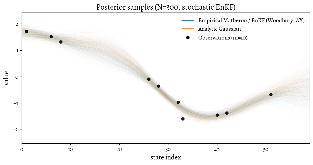
2 Demo

Here we do three things:

1. build a simple 1D GP prior (a squared‑exp kernel over a grid),
2. generate a single “truth” and a noisy observation \(y^*\) at a handful of points,
3. draw an empirical posterior ensemble via the Matheron/EnKF rule and check it against the analytic Gaussian posterior.

Code

import numpy as np
import matplotlib.pyplot as plt
from matplotlib.lines import Line2D
from livingthing.matplotlib_style import set_livingthing_style, reset_default_style

set_livingthing_style()

rng = np.random.default_rng(11)

# Dimensions
d, m, N = 60, 10, 300

# Prior: squared-exponential on a 1D grid
def se_cov(n, ell=12.0, sigma=1.0, jitter=1e-8):
    x = np.arange(n)[:, None]
    S = sigma**2 * np.exp(-0.5 * (x - x.T)**2 / ell**2)
    return S + jitter*np.eye(n)

m0 = np.zeros(d)
Sigma = se_cov(d, ell=12.0, sigma=1.0)
L = np.linalg.cholesky(Sigma)

# Observation operator (m point picks) and noise
idx = np.sort(rng.choice(d, size=m, replace=False))
H = np.zeros((m, d)); H[np.arange(m), idx] = 1.0
rho = 0.15
R = (rho**2) * np.eye(m)

# One truth and its noisy observations
x_true = m0 + L @ rng.standard_normal(d)
y_star = H @ x_true + rho * rng.standard_normal(m)

# Prior ensemble
X = m0[:, None] + L @ rng.standard_normal((d, N))

# Choose EnKF flavour
stochastic = True  # True: perturbed obs; False: deterministic/square-root

if stochastic:
    Eps = rho * rng.standard_normal((m, N))
    Y = H @ X + Eps
    gamma_diag = 1e-9 * np.ones(m)   # only tiny ridge (R already inside sample cov through Y)
else:
    Y = H @ X
    gamma_diag = np.diag(R) + 1e-9

# Centered ensembles
Xc = X - X.mean(axis=1, keepdims=True)   # d x N
Yc = Y - Y.mean(axis=1, keepdims=True)   # m x N

# Woodbury factors
sqrtN1 = np.sqrt(N - 1.0)
U = Yc / sqrtN1                          # m x N
Gamma_inv = 1.0 / gamma_diag             # length-m

# residuals in obs space
Res = (y_star[:, None] - Y)              # m x N

# Build A = U^T Γ^{-1} U (N x N) and B = U^T Γ^{-1} Res (N x N) efficiently
U_over_Gamma = U * Gamma_inv[:, None]    # m x N (diag multiply)
A = U.T @ U_over_Gamma                   # N x N
B = U.T @ (Res * Gamma_inv[:, None])     # N x N

# Solve (I + A) Q = B  for Q, then ΔX = (1/sqrt(N-1)) Xc @ Q
I_N = np.eye(N)
M = np.linalg.inv(I_N + A)
Q = M @ B                                # N x N
dX = (Xc @ Q) / sqrtN1                   # d x N

X_post_enkf = X + dX

# Analytic posterior ensemble for comparison
S = H @ Sigma @ H.T + R
K = Sigma @ H.T @ np.linalg.inv(S)
mu_post = m0 + K @ (y_star - H @ m0)
Sigma_post = Sigma - K @ H @ Sigma
L_post = np.linalg.cholesky(Sigma_post + 1e-9*np.eye(d))
X_post_analytic = mu_post[:, None] + L_post @ rng.standard_normal((d, N))

# Plotting (single axes)
alpha = float(N)**(-0.75)
alpha = max(min(alpha, 0.25), 0.003)
x_axis = np.arange(d)

c_enkf     = 'tab:blue'
c_analytic = 'tab:orange'
c_obs      = 'black'

y_min = min(X_post_enkf.min(), X_post_analytic.min(), y_star.min())
y_max = max(X_post_enkf.max(), X_post_analytic.max(), y_star.max())
pad = 0.05*(y_max - y_min + 1e-12)
ylims = (y_min - pad, y_max + pad)

plt.figure(figsize=(9, 4.8), dpi=120)
for i in range(N):
    plt.plot(x_axis, X_post_enkf[:, i], color=c_enkf, alpha=alpha, linewidth=1.0)
    plt.plot(x_axis, X_post_analytic[:, i], color=c_analytic, alpha=alpha, linewidth=1.0)
plt.scatter(idx, y_star, s=32, color=c_obs, marker='o', alpha=0.9, zorder=3)

proxy_enkf = Line2D([0], [0], color=c_enkf,     lw=2, alpha=0.9, label='Empirical Matheron / EnKF (Woodbury, ΔX)')
proxy_an   = Line2D([0], [0], color=c_analytic, lw=2, alpha=0.9, label='Analytic Gaussian')
proxy_obs  = Line2D([0], [0], color=c_obs, marker='o', lw=0, label='Observations (m=10)')
plt.legend(handles=[proxy_enkf, proxy_an, proxy_obs], loc='upper right', frameon=False)

plt.title(f'Posterior samples (N={N}, {"stochastic" if stochastic else "deterministic"} EnKF)')
plt.xlabel('state index')
plt.ylabel('value')
plt.ylim(*ylims)
plt.xlim(0, d-1)
plt.tight_layout()
plt.show()

# Quick numeric check
mean_rel_err = np.linalg.norm(X_post_enkf.mean(axis=1) - mu_post) / (np.linalg.norm(mu_post) + 1e-12)
cov_rel_err  = np.linalg.norm(np.cov(X_post_enkf, bias=False) - Sigma_post, 'fro') / (np.linalg.norm(Sigma_post, 'fro') + 1e-12)
print("Relative mean error (EnKF vs analytic):", f"{mean_rel_err:.3e}")
print("Relative cov  error (EnKF vs analytic):", f"{cov_rel_err:.3e}")

Relative mean error (EnKF vs analytic): 5.756e-02
Relative cov  error (EnKF vs analytic): 8.156e-02

3 How to read it

• Everything is standard linear‑Gaussian conditioning; the only twist is that we replace true covariances with ensemble covariances.
• With a noisy observation ensemble \(Y=HX+\varepsilon\), the empirical \(C_{yy}\) already contains \(R\); don’t add it again.
• With a noise‑free observation ensemble \(Y=HX\), add \(R\) explicitly to \(\widehat C_{yy}\) (and we’ll typically use a square‑root transform to update the ensemble).

4 Why I care

• It gives a pathwise sampler: we obtain samples by an affine residual correction—no Cholesky of the posterior needed.
• It unifies toolboxes: localization, inflation, and square‑root tricks from EnKF port straight over to pathwise GP sampling; conversely, autodiff and sparse‑GP ideas go the other way.
• It clarifies the zoo: stochastic EnKF and conditional GP all share the same core update; the differences are entirely in how we build \(\widehat C\) and whether we perturb \(y\).

I particularly care because we’re moving towards the world of generative AI. These days we work with samples, not densities.

If what we actually need are posterior samples, the Matheron/EnKF rule is the “right thing”: it’s an affine pushforward that maps a prior draw \(x\) to a posterior draw \(x' = x + C_{xy}C_{yy}^{-1}(y^\* - y)\). It avoids building or storing any \(d\times d\) covariance at all; it only needs matrix–vector products with \(H\), performs solves in the observation space, and gives us Monte‑Carlo access to any posterior functional we care about. In other words, computing the full posterior covariance isn’t just expensive for large \(d\); it’s usually irrelevant. The sample-to-sample map is also a reparameterization, so it’s differentiable and streams naturally as new data arrive (update the same ensemble, don’t refactor a giant matrix). We can treat the posterior as a set of paths, not a density we must summarize, and the implementation choices present themselves. See the toy code path for a minimal demonstration of this empirical posterior sampler.

5 Implications

Understanding the EnKF as an empirical Matheron update opens up several possibilities. Both the Matheron update and Ensemble Kalman methods have been extensively studied in their respective fields. In recent years, numerous developments in Bayesian machine learning have advanced both approaches; see the many developments in Ensemble Kalman methods in the Ensemble Kalman notebook and especially the Neural networks meet Kalman filters notebook.

If we interpret the pathwise Matheron update in the context of the empirical measures used in the EnKF, this suggests we can import developments from one field to the other. The vast literature on the EnKF indicates that many ideas developed there might be applicable to Gaussian Process regression via the Matheron update. For instance, the clear probabilistic interpretation of the ensemble update could inspire improved regularization and localization strategies. One example is the Local Ensemble Transform Kalman Filter (Bocquet, Farchi, and Malartic 2020), which provides state‑of‑the‑art performance in high-dimensional filtering and system identification settings and could be adapted to the Matheron update (homework exercise).

@inproceedings{MacKinlay2025Ensemble,
  title = {The {{Ensemble Kalman Update}} Is an {{Empirical Matheron Update}}},
  booktitle = {Australian {{Joint Conference}} on {{AI}}},
  author = {MacKinlay, Dan},
  year = 2025,
  month = dec,
  series = {Lecture Note on {{Computer Science}}},
  publisher = {Springer},
  address = {Canberra},
  doi = {10.48550/arXiv.2502.03048},
  archiveprefix = {arXiv}
}

6 Appendix: the deterministic (square‑root) variant in one line

If we prefer not to perturb the observations, set \(Y=HX\) and use

\[ K=\widehat C_{xy}\,\bigl(\widehat C_{yy} + R\bigr)^{-1}. \]

This matches the posterior mean and covariance. To produce an actual posterior sample, we need to use an ensemble transform (ETKF/LETKF, etc.) rather than the residual‑add form above.

7 References