Posterior Gaussian process samples by updating prior samples

1 Matheron updates for Gaussian RVs

We start by examining a slightly different way of defining a Gaussian RV (J. T. Wilson et al. 2021) starting from the recipe for sampling:

A random vector \(\boldsymbol{x}=\left(x_{1}, \ldots, x_{n}\right) \in \mathbb{R}^{n}\) is said to be Gaussian if there exists a matrix \(\mathbf{L}\) and vector \(\boldsymbol{\mu}\) such that \[ \boldsymbol{x} \stackrel{\mathrm{d}}{=} \boldsymbol{\mu}+\mathbf{L} \boldsymbol{\zeta} \quad \boldsymbol{\zeta} \sim \mathcal{N}(\mathbf{0}, \mathbf{I}) \] where \(\mathcal{N}(\mathbf{0}, \mathbf{I})\) is known as the standard version of a (multivariate) normal distribution, which is defined through its density.

This is the location-scale form of a Gaussian RV, as opposed to the canonical form which we use in Gaussian Belief Propagation. In location-scale form, a non-degenerate Gaussian RV’s distribution is given (uniquely) by its mean \(\boldsymbol{\mu}=\mathbb{E}(\boldsymbol{x})\) and its covariance \(\boldsymbol{\Sigma}=\mathbb{E}\left[(\boldsymbol{x}-\boldsymbol{\mu})(\boldsymbol{x}-\boldsymbol{\mu})^{\top}\right] .\) In this notation the density, if defined, is \[ p(\boldsymbol{x})=\mathcal{N}(\boldsymbol{x} ; \boldsymbol{\mu}, \boldsymbol{\Sigma})=\frac{1}{\sqrt{|2 \pi \boldsymbol{\Sigma}|}} \exp \left(-\frac{1}{2}(\boldsymbol{x}-\boldsymbol{\mu})^{\top} \boldsymbol{\Sigma}^{-1}(\boldsymbol{x}-\boldsymbol{\mu})\right). \]

Since \(\zeta\) has identity covariance, any matrix square root of \(\boldsymbol{\Sigma}\), such as the Cholesky factor \(\mathbf{L}\) with \(\boldsymbol{\Sigma}=\mathbf{L L}^{\top}\), may be used to draw \(\boldsymbol{x}=\boldsymbol{\mu}+\mathbf{L} \boldsymbol{\zeta}.\)

tl;dr we can think about drawing any Gaussian RV as transforming a standard Gaussian. So much is basic entry-level stuff. What might a rule which updates a Gaussian prior into a data-conditioned posterior look like? Like this!

We define \(\cov(a,b)=\Sigma_{a,b}\) as the covariance between two random variables (J. T. Wilson et al. 2021):

Matheron’s Update Rule: Let \(\boldsymbol{a}\) and \(\boldsymbol{b}\) be jointly Gaussian, centered random variables. Then the random variable \(\boldsymbol{a}\) conditional on \(\boldsymbol{b}=\boldsymbol{\beta}\) may be expressed as \[ (\boldsymbol{a} \mid \boldsymbol{b}=\boldsymbol{\beta}) \stackrel{\mathrm{d}}{=} \boldsymbol{a}+\boldsymbol{\Sigma}_{\boldsymbol{a}, \boldsymbol{b}}{\boldsymbol{\Sigma}}_{\boldsymbol{b}, \boldsymbol{b}}^{-1}(\boldsymbol{\beta}-\boldsymbol{b}) \] Proof: Comparing the mean and covariance on both sides immediately affirms the result \[ \begin{aligned} \mathbb{E}\left(\boldsymbol{a}+\boldsymbol{\Sigma}_{\boldsymbol{a}, \boldsymbol{b}} \boldsymbol{\Sigma}_{\boldsymbol{b}, \boldsymbol{b}}^{-1}(\boldsymbol{\beta}-\boldsymbol{b})\right) & =\boldsymbol{\mu}_{\boldsymbol{a}}+\boldsymbol{\Sigma}_{\boldsymbol{a}, \boldsymbol{b}} \boldsymbol{\Sigma}_{\boldsymbol{b}, \boldsymbol{b}}^{-1}\left(\boldsymbol{\beta}-\boldsymbol{\mu}_{\boldsymbol{b}}\right) \\ & =\mathbb{E}(\boldsymbol{a} \mid \boldsymbol{b}=\boldsymbol{\beta}) \end{aligned} \] \[ \begin{aligned} \operatorname{Cov}\left(\boldsymbol{a}+\boldsymbol{\Sigma}_{\boldsymbol{a}, \boldsymbol{b}} \boldsymbol{\Sigma}_{\boldsymbol{b}, \boldsymbol{b}}^{-1}(\boldsymbol{\beta}-\boldsymbol{b})\right) &=\boldsymbol{\Sigma}_{\boldsymbol{a}, \boldsymbol{a}}+\boldsymbol{\Sigma}_{\boldsymbol{a}, \boldsymbol{b}} \boldsymbol{\Sigma}_{\boldsymbol{b}, \boldsymbol{b}}^{-1} \operatorname{Cov}(\boldsymbol{b}) \boldsymbol{\Sigma}_{\boldsymbol{b}, \boldsymbol{b}}^{-1} \boldsymbol{\Sigma}_{\boldsymbol{b}, \boldsymbol{a}} \\ & =\boldsymbol{\Sigma}_{\boldsymbol{a}, \boldsymbol{a}}+\boldsymbol{\Sigma}_{\boldsymbol{a}, \boldsymbol{b}} \boldsymbol{\Sigma}_{\boldsymbol{b}, \boldsymbol{b}}^{-1} \boldsymbol{\Sigma}_{\boldsymbol{b}, \boldsymbol{a}}\\ &=\operatorname{Cov}(\boldsymbol{a} \mid \boldsymbol{b} =\boldsymbol{\beta}) \end{aligned} \]

Can we find a transformation that will turn a Gaussian process prior sample (i.e. function) into a Gaussian process posterior sample, and thus use prior samples, which are presumably pretty easy, to create posterior ones, which are often hard. If we evaluate the sampled function at a finite number of points, then we can use the Matheron formula to do precisely that. Sometimes this can even be useful. The resulting algorithm uses tricks from both analytic GP regression and Monte Carlo.

The sample based approximation to this is precisely the Ensemble Kalman Filter.

2 “Exact” updates for Gaussian processes

Exact in the sense that we do not approximate the data. These updates are not exact if our basis function representation is only an approximation to the “true” GP (as with classic GPs) and not exact in the sense that we will be using samples to approximate measures. For now we assume that the observation likelihood is Gaussian.¹

For a Gaussian process \(f \sim \mathcal{G P}(\mu, k)\) with marginal \(\boldsymbol{f}_{m}=f(\mathbf{Z})\), the process conditioned on \(\boldsymbol{f}_{m}=\boldsymbol{y}\) admits, in distribution, the representation \[ \underbrace{(f \mid \boldsymbol{y})(\cdot)}_{\text {posterior }} \stackrel{\mathrm{d}}{=} \underbrace{f(\cdot)}_{\text {prior }}+\underbrace{k(\cdot, \mathbf{Z}) \mathbf{K}_{m, m}^{-1}\left(\boldsymbol{y}-\boldsymbol{f}_{m}\right)}_{\text {update }}. \]

If our observations are contaminated by additive i.i.d Gaussian noise, \(\boldsymbol{y}=\boldsymbol{f}_{m} +\boldsymbol{\varepsilon}\) with \(\boldsymbol{\varepsilon}\sim\mathcal{N}(\boldsymbol{0}, \sigma^2\mathbf{I}),\) we find \[ \begin{aligned} &\boldsymbol{f}_{*} \mid \boldsymbol{y} \stackrel{\mathrm{d}}{=} \boldsymbol{f}_{*}+\mathbf{K}_{*, n}\left(\mathbf{K}_{n, n}+\sigma^{2} \mathbf{I}\right)^{-1}(\boldsymbol{y}-\boldsymbol{f}-\boldsymbol{\varepsilon}) \end{aligned} \] When sampling from exact GPs we jointly draw \(\boldsymbol{f}_{*}\) and \(\boldsymbol{f}\) from the prior. Then, we combine \(\boldsymbol{f}\) with noise variates \(\varepsilon \sim \mathcal{N}\left(\mathbf{0}, \sigma^{2} \mathbf{I}\right)\) such that \(\boldsymbol{f}+\varepsilon\) constitutes a draw from the prior distribution of \(\boldsymbol{y}\).

Compare this to the equivalent distributional update from classical GP regression which updates the moments of a distribution, not samples from a path — the formulae are related though:

…the conditional distribution is the Gaussian \(\mathcal{N}\left(\boldsymbol{\mu}_{* \mid y}, \mathbf{K}_{*, * \mid y}\right)\) with moments \[\begin{aligned} \boldsymbol{\mu}_{* \mid \boldsymbol{y}}&=\boldsymbol{\mu}_*+\mathbf{K}_{*, n} \mathbf{K}_{n, n}^{-1}\left(\boldsymbol{y}-\boldsymbol{\mu}_n\right) \\ \mathbf{K}_{*, * \mid \boldsymbol{y}}&=\mathbf{K}_{*, *}-\mathbf{K}_{*, n} \mathbf{K}_{n, n}^{-1} \mathbf{K}_{n, *}\end{aligned} \]

3 Using basis functions

For many purposes we need a basis function representation, a.k.a. the weight-space representation. We assert the GP can be written as a random function comprising basis functions \(\boldsymbol{\phi}=\left(\phi_{1}, \ldots, \phi_{\ell}\right)\) with the Gaussian random weight vector \(w\) so that \[ f^{(w)}(\cdot)=\sum_{i=1}^{\ell} w_{i} \phi_{i}(\cdot) \quad \boldsymbol{w} \sim \mathcal{N}\left(\mathbf{0}, \boldsymbol{\Sigma}_{\boldsymbol{w}}\right). \] \(f^{(w)}\) is a random function satisfying \(\boldsymbol{f}^{(\boldsymbol{w})} \sim \mathcal{N}\left(\mathbf{0}, \boldsymbol{\Phi}_{n} \boldsymbol{\Sigma}_{\boldsymbol{w}} \boldsymbol{\Phi}^{\top}\right)\), where \(\boldsymbol{\Phi}_{n}=\boldsymbol{\phi}(\mathbf{X})\) is a \(|\mathbf{X}| \times \ell\) matrix of features. If we are lucky, the representation might not be too bad when the basis is truncated to a small size.

The posterior weight distribution \(\boldsymbol{w} \mid \boldsymbol{y} \sim \mathcal{N}\left(\boldsymbol{\mu}_{\boldsymbol{w} \mid n}, \boldsymbol{\Sigma}_{\boldsymbol{w} \mid n}\right)\) is Gaussian with moments \[ \begin{aligned} \boldsymbol{\mu}_{\boldsymbol{w} \mid n} &=\left(\boldsymbol{\Phi}^{\top} \boldsymbol{\Phi}+\sigma^{2} \mathbf{I}\right)^{-1} \boldsymbol{\Phi}^{\top} \boldsymbol{y} \\ \boldsymbol{\Sigma}_{\boldsymbol{w} \mid n} &=\left(\boldsymbol{\Phi}^{\top} \boldsymbol{\Phi}+\sigma^{2} \mathbf{I}\right)^{-1} \sigma^{2} \end{aligned} \] where \(\boldsymbol{\Phi}=\boldsymbol{\phi}(\mathbf{X})\) is an \(n \times \ell\) feature matrix. We solve for the right-hand side at \(\mathcal{O}\left(\min \{\ell, n\}^{3}\right)\) cost by applying the Woodbury identity as needed. So far there is nothing unusual here; the cool bit is realising we can represent this update as an independent operation.

In the weight-space setting, the pathwise update given an initial weight vector \(\boldsymbol{w} \sim \mathcal{N}(\mathbf{0}, \mathbf{I})\) is \(\boldsymbol{w} \mid \boldsymbol{y} \stackrel{\mathrm{d}}{=} \boldsymbol{w}+\boldsymbol{\Phi}^{\top}\left(\boldsymbol{\Phi} \boldsymbol{\Phi}^{\top}+\sigma^{2} \mathbf{I}\right)^{-1}\left(\boldsymbol{y}-\boldsymbol{\Phi}^{\top} \boldsymbol{w}-\boldsymbol{\varepsilon}\right).\)

So if we had a nice weight-space representation for everything already we could go home at this point. However, for many models we are not given that; we might find natural bases for the prior and posterior are not the same (the posterior should not be stationary usually, for one thing).

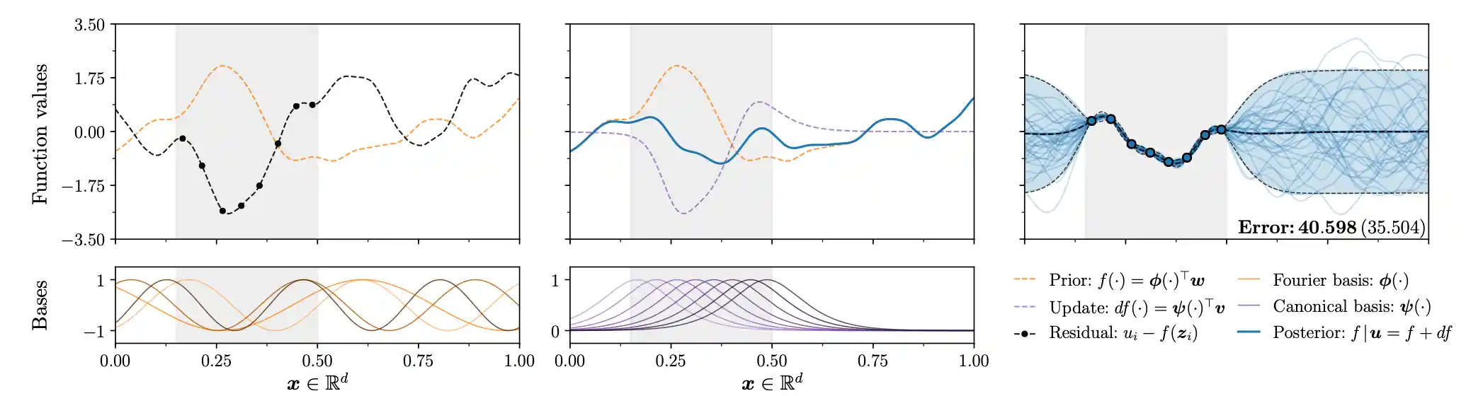
The innovation in J. T. Wilson et al. (2020) is to make different choices of functional bases for prior and posterior updates. We can choose anything really, AFAICT. They suggest Fourier basis for prior and the canonical basis, i.e. the reproducing kernel basis \(k(\cdot,\vv{x})\) for the update. Then we have \[ \underbrace{(f \mid \boldsymbol{y})(\cdot)}_{\text {sparse posterior }} \stackrel{\mathrm{d}}{\approx} \underbrace{\sum_{i=1}^{\ell} w_{i} \phi_{i}(\cdot)}_{\text {weight-space prior}} +\underbrace{\sum_{j=1}^{m} v_{j} k\left(\cdot, \boldsymbol{x}_{j}\right)}_{\text {function-space update}} , \] where we have defined \(\boldsymbol{v}=\left(\mathbf{K}_{n, n}+\sigma^{2} \mathbf{I}\right)^{-1}\left(\boldsymbol{y}-\boldsymbol{\Phi}^{\top} \boldsymbol{w}- \boldsymbol{\varepsilon}\right) .\)

4 Sparse GP setting

I.e. using inducing variables.

Given \(q(\boldsymbol{u})\), we approximate posterior distributions as \[ p\left(\boldsymbol{f}_{*} \mid \boldsymbol{y}\right) \approx \int_{\mathbb{R}^{m}} p\left(\boldsymbol{f}_{*} \mid \boldsymbol{u}\right) q(\boldsymbol{u}) \mathrm{d} \boldsymbol{u} . \] If \(\boldsymbol{u} \sim \mathcal{N}\left(\boldsymbol{\mu}_{\boldsymbol{u}}, \boldsymbol{\Sigma}_{\boldsymbol{u}}\right)\), we compute this integral analytically to obtain a Gaussian distribution with mean and covariance \[ \begin{aligned} \boldsymbol{m}_{* \mid m} &=\mathbf{K}_{*, m} \mathbf{K}_{m, m}^{-1} \boldsymbol{\mu}_{m} \\ \mathbf{K}_{*, * \mid m} &=\mathbf{K}_{*, *}+\mathbf{K}_{*, m} \mathbf{K}_{m, m}^{-1}\left(\boldsymbol{\Sigma}_{\boldsymbol{u}}-\mathbf{K}_{m, m}\right) \mathbf{K}_{m, m}^{-1} \mathbf{K}_{m, *^{*}} \end{aligned} \]

\[ \begin{aligned} &\boldsymbol{f}_{*} \mid \boldsymbol{u} \stackrel{\mathrm{d}}{=} \boldsymbol{f}_{*}+\mathbf{K}_{*, m} \mathbf{K}_{m, m}^{-1}\left(\boldsymbol{u}-\boldsymbol{f}_{m}\right) \\ \end{aligned} \]

When sampling from sparse GPs we draw \(\boldsymbol{f}_{*}\) and \(\boldsymbol{f}_{m}\) together from the prior, and independently generate target values \(\boldsymbol{u} \sim q(\boldsymbol{u}) .\) \[ \underbrace{(f \mid \boldsymbol{u})(\cdot)}_{\text {sparse posterior }} \stackrel{\mathrm{d}}{\approx} \underbrace{\sum_{i=1}^{\ell} w_{i} \phi_{i}(\cdot)}_{\text {weight-space prior}} +\underbrace{\sum_{j=1}^{m} v_{j} k\left(\cdot, \boldsymbol{z}_{j}\right)}_{\text {function-space update}} , \] where we have defined \(\boldsymbol{v}=\mathbf{K}_{m, m}^{-1}\left(\boldsymbol{u}-\boldsymbol{\Phi}^{\top} \boldsymbol{w}\right) .\)

5 Matrix GPs

(Ritter et al. 2021 appendix D) reframes the Matheron update and generalises it to matrix-Gaussians. TBC.

6 Stationary moves

Thus far we have talked about moves updating a prior to a posterior; how about moves within a posterior?

We could try Langevin sampling, for example, or SG MCMC but these all seem to require inverting the covariance matrix so are not likely to be efficient in general. Can we do better?

7 Incoming

• Alexander Terenin, Pathwise Conditioning and Non-Euclidean Gaussian Processes

8 References