Isotropic random vectors

1 Simulating isotropic vectors

Let’s say you wish to simulate a random variable, $X$ whose realisations are isotropically distributed unit-vectors (say, to represent isotropic rotations, or for a null-distribution against which to check for isotropy.)

The simplest way I know of generating such vectors is to take $$X\sim \mathcal{N}({\mathbf{0}}_d,{\mathbf{I}}_d)$$

That is, $X$ distributed by a multivariate Gaussian distribution with each component independent and of standard deviation 1, so if $X_i$ are i.i.d. with $X_i\sim \mathcal{N}(0,1)$, then $$X=\left[\begin{array}{c}{X}_1\\ X_2\\ ⋮\\ X_d\end{array}\right]$$

By the rotational invariance of multivariate Gaussian distributions, we know that this must be isotropic.

Update: Martin Roberts collects a bumper list, How to generate uniformly random points on n-spheres and in n-balls. There are some surprising ones.

2 Marginal distributions

Question: what is the marginal distribution of the axial component $U_i$, of $U$, along axis $i$, in the non-trivial case with $d>1$?

Let us consider, w.l.o.g., $U_1$. We know that the p.d.f of $U_1$ is even (i.e. has reflective symmetry) by construction. So it will suffice to find the positive half of the distribution function. Thus it will also be enough to find the p.d.f. of $U_1^2$.

Define $$X^{\prime }\equiv \left[\begin{array}{c}{X}_2\\ X_3\\ ⋮\\ X_d\end{array}\right]$$ i.e. $X^{\prime }$ is $X$ with the first component of the vector excised. We have $$\begin{array}{cccc}& U& =& \frac{X}{\Vert X\Vert }\\ \Rightarrow & U^2& =& \frac{X^2}{{\Vert X\Vert }^2}\\ \Rightarrow & U_1^2& =& \frac{X_1^2}{{\Vert X\Vert }^2}\\ \Rightarrow & U_1^2& =& \frac{X_1^2}{{\Vert X^{\prime }\Vert }^2+X_1^2}\\ \Rightarrow & \frac{1}{U_1^2}-1& =& \frac{{\Vert X^{\prime }\Vert }^2}{X_1^2}\\ \Rightarrow & \frac{\frac{1}{U_1^2}-1}{d-1}& =& \frac{{\Vert X^{\prime }\Vert }^2/(d-1)}{X_1^2}\end{array}$$

Now, the R.H.S. has an $\mathcal{F}(d-1,1)$ distribution, as the ratio of i.i.d ${\chi }^2$ variables, and the work there has already been done for us by Snedecor. We call that R.H.S. $G$, where $G\sim \mathcal{F}(d-1,1)$. We write $g$ for the pdf. Then $$U_1^2=\frac{1}{g(d-1)+1}$$

Now we can construct the pdf of $U_1$. In fact, for my purposes I need the quantile/inverse-cdf function, so let’s do that. Call the quantile function of the $\mathcal{F}(d-1,1)$ distribution, $H(x)$ and the cdf of $U_1$, $F(x)$ (for ‘half’ and ‘full’).

Then we splice two symmetric copies of the function about the axis — $F(x)=\mathrm{sgn}(2x-1)H(1-|2x-1|)$ - and we’re done.

Here’s a plot of the behaviour of our distribution:

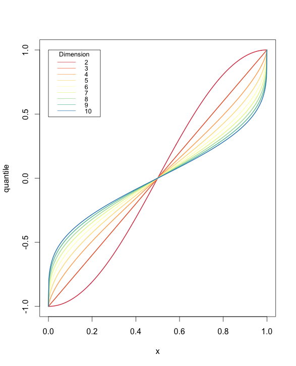
Notice that axial components tend to be long in ${\mathbb{R}}^2$, and short in more than 3 dimensions. And uniformly distributed in 3 dimensions. Intuitively, as the number of dimensions increases, the contribution of any one axis to the total length is likely to be smaller on average, because there are simply more of them.

And here’s the R code to generate the graph, most of which is plotting logic.

half.quantile <- function(x,d=3) {
    g <- qf(x,d-1,1)
    return(1/sqrt(g*(d-1)+1))
}
full_quantile <- function (x, d=3) {
    x.scaled <- 2*x -1
    res <- sign(x.scaled)*half.quantile(1-abs(x.scaled), d)
    return(res)
}

pts <- seq(0,1,1/512)
dims <- seq(2,10)
ndims <- length(dims)
vals <- data.frame(outer(pts, dims, full.quantile))
dimnames <- paste(dims)
xrange <- c(0,1)
yrange <- c(-1,1)
library(RColorBrewer)
colors <- brewer.pal(ndims,"Spectral")

# set up the plot
plot(xrange, yrange, type="l", xlab="x",
        ylab="quantile")

# add lines
for (i in seq(ndims)) {
    dim <- vals[,i]
    lines(pts, dim, type="l", lwd=2,
    col=colors[i],
    lty=1
    )
}

# add a legend
legend(xrange[1], yrange[2], dims, cex=0.8, col=colors,
        lty=1, title="Dimension")

There are many interesting approximate distributions for these quantities, which are explored in the low-d projections notebook.

3 Inner products

There is an exact distribution for inner products of normalized vectors. Suppose that $L=\frac{1}{2}+\text{vv}{X}_p^{\mathrm{\top }}\text{vv}{X}_q/2$. Then $L\sim \mathrm{Beta}((D-1)/2,(D-1)/2).$

4 Moments

Kimchi lover derives the variance of $x_i$ chosen uniformly from the hypersphere:

$$\mathit{x}\sim \mathrm{Unif}{\mathbb{B}}^{d-1}\Rightarrow \mathrm{Var}(X_1)=\frac{1}{d+2}.$$

See also Covariance matrix of uniform spherical distribution wherein a very simple symmetry argument gives $$\mathit{x}\sim \mathrm{Unif}{\mathbb{S}}^{d-1}\Rightarrow \mathrm{Var}(X_1)=\frac{1}{d}.$$ and indeed $$\mathit{x}\sim \mathrm{Unif}{\mathbb{S}}^{d-1}\Rightarrow \mathrm{Var}(\mathit{x})=\frac{1}{d}\mathrm{I}.$$

5 Archimedes Principles

First mention: The first $(n-2)$ coordinates on a sphere are uniform in a ball

Djalil Chafaï mentions the Archimedes principle which

… states that the projection of the uniform law of the unit sphere of ${\mathbb{R}}^3$ on a diameter is the uniform law on the diameter. It is the case $n=3$ of the Funk-Hecke formula…. More generally, if $(X_1,\dots ,X_n)$ is a random vector of ${\mathbb{R}}^n$ uniformly distributed on the unit sphere ${\mathbb{S}}^{n-1}$ then $(X_1,\dots ,X_{n-2})$ is uniformly distributed on the unit ball of ${\mathbb{R}}^{n-2}$. It does not work if we replace $n-2$ by $n-1$.

6 Funk-Hecke

Djalil Chafaï introduces the The Funk-Hecke formula:

In its basic form, the Funk-Hecke formula states that for all bounded measurable $f:[-1,1]\mapsto \mathbb{R}$ and all $y\in {\mathbb{S}}^{n-1}$, $$\int f(x\cdot y){\sigma }_{{\mathbb{S}}^{n-1}}(\mathrm{d}x)=\frac{\mathrm{\Gamma }\left(\frac{n}{2}\right)}{\sqrt{\pi }\mathrm{\Gamma }\left(\frac{n-1}{2}\right)}{\int }_{-1}^{1}f(t){(1-t^2)}^{\frac{n-3}{2}}\mathrm{d}t$$ The formula does not depend on $x$, an invariance due to spherical symmetry.…

If this is an inner product with a sphere RV then we get the density for a univariate random projection.

7 References