Musical metrics and manifolds
2014-09-26 — 2017-03-27
Wherein musical spaces, metrics and kernels are considered, Plomp and Levelt’s dissonance curves are invoked to induce nearly circular geometries which are shown to recover the equal‑tempered 12‑tone scale.
Metrics, kernels and affinities and the spaces and topologies they induce and what they reveal (or prescribe) about composition. This has considerable overlap with machine listening, but there I start from audio signals, and here I usually think about more “symbolic” data such as musical scores, and with rhythm, but there I care only about the time axis. There is overlap also with psychoacoustic units and auditory features which are the pure elements from which these amalgams are made.
One thing which has become outdated in this notebook since I wrote it is that these days I would naturally consider learned metrics, rather than a priori ones.
This is a specialised area with many fine careers built on it, and many schools with long and proud histories of calling adherents of other schools wrong. A short literature search will find many worth distinctions drawn between differences, cultural versus the biological, general versus individual, the different models applicable at different time scales, of masking effects and such.
I will pass over these fine contrasts without note, in my quest for some pragmatically useful, minimally complex features for use in machine-learning algorithms, which do not require truth but functionality.
See also machine listening, Arpeggiate by Numbers, clustering, manifold learning.
1 General musically-motivated metric spaces
Chords etc.
Consider grouping chords played on a piano with some known (idealised) 16-harmonic spectrum. How can we understand the harmonic relations of chords played upon this keyboard?
We know a-priori that this projection can be naturally embedded in a Euclidean space with something less than \(16\times 12 = 192\) dimensions, since there are at most that many spectral bands. In fact, since there are only 12 notes, we can get this down to 12 dimensions. The question is, can we get to an even smaller number of dimensions? How small? By “small” here, I mean, can I group chords on a lower number of dimensions than this in some musically interesting way? For bonus points, can I group chords into several different such maps and switch between them?
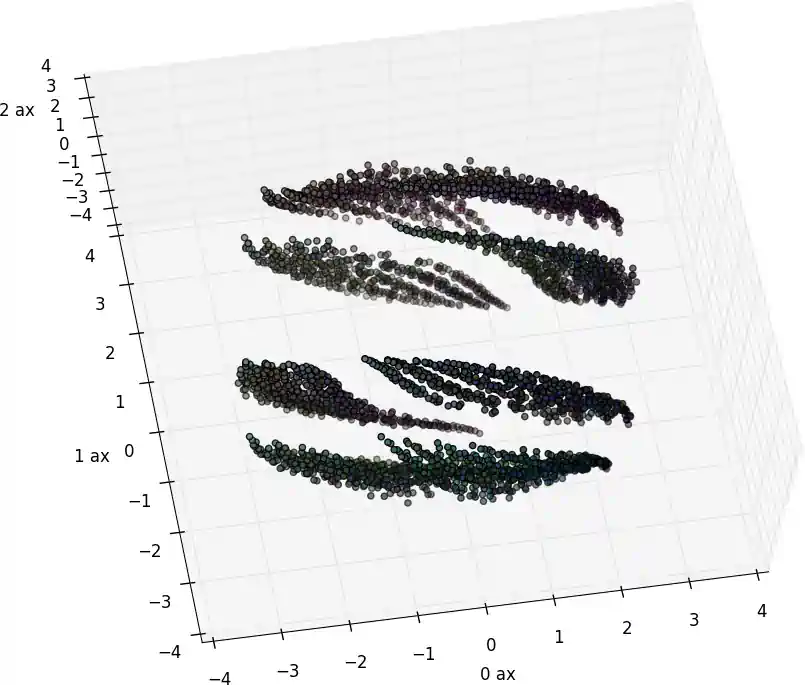
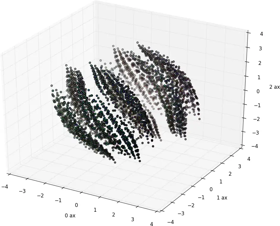
Without explanation, here is one similarity-distance embedding of all the chords using an ad hoc metric based on thinking about this question. (Brightness: The more notes in the chord, the darker. Hue: I forget.)
Question: can we use word-bag models for note adjacency representation? Since I asked that question I discovered the Chord2vec model of Walder’s lab, whose answer is “yes”. See Madjiheurem, Qu, and Walder (2016).
2 To understand
Basic group theory: What are the symmetries of the group of all pitch class co-occurrences in the 12-tet? The most common pitch class co-occurrence is a 12-vector over the Boolean algebra where a “1” in the first entry means “the note C was played”, in pos 2, “C-sharp was played” etc. Symmetries we care about are, for example, that (under equal temperament) chord harmonic relationships should be invariant under transposition — i.e. rotation of the entries of the vector. (this last is not so in the case of Sethares/Terhardt style dissonance theory, which considers only unwrapped harmonics.)
Dmitri Tymoczko’s Geometrical Methods in Recent Music Theory
Henjan Honing’s Musical Cognition: any good?
3 Dissonance
a.k.a. “Spectral roughness”. A particular empirically-motivated metric, with good predictive performance despite its simplicity, and wilful lack of concern for the actual mechanisms of the ear and the brain, or modern nuances such as masking effects and the influence of duration on sound perception etc. Invented by Plomp and Levelt (Plomp and Levelt 1965), and developed by variously, Sethares, Terhardt and Parncutt and others.
Some sources seem to distinguish roughness in the sense of Sethares from the Plomp and Levelt sense, although they use qualitatively equations. I suspect therefore that the distinction is philosophical, or possibly pointed failure to cite one another because someone said something rude at the after-conference drinkies.
An overview by Vassilakis might help, or the app based on his work by Dr Kelly Fitz.
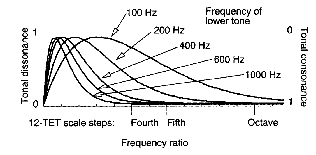
Plomp and Levelt’s dissonance curves ((Plomp and Levelt 1965; Sethares 1997)).
Juan Sebastian Lach Lau produced some actual open-source software (DissonanceLib) that attempts to action this stuff in a musical setting. There is a slightly different version below attributed to Parncutt.
A convenient summary of both is in the DissonanceLib code.
It’s most useful for things where you are given the harmonics a priori; I’m not especially convinced about the tenability of directly inferring this metric from an audio signal (“how dissonant is this signal?”). We should be cautious about the identifiability of this statistic from signals nonparametrically e.g. windowed DTFT power-spectrogram peaks, just because beat frequency stuff is complicated and runs into the uncertainty principle. (Terhardt, Stoll, and Seewann 1982; Sethares 1998b) give it a go, though. Inferring dissonance between two signals known to be not dissonant might work though, or perhaps one might need parametric approaches, as in linear system identification
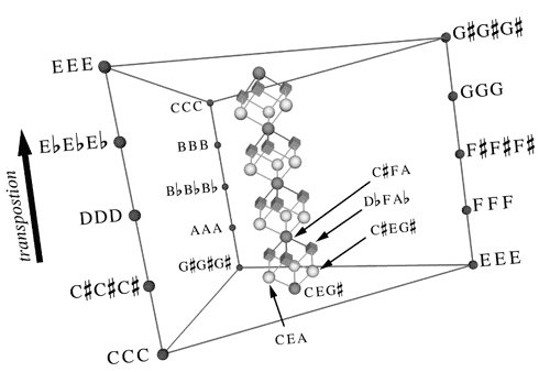
Dissonance is an interesting measure, despite these problems, though because it is very much like a Mercer kernel, in that it constructs a distance defined on an (explicit) high-dimensional space; Also, the “nearly circular” geometry it induces is interesting; For harmonic spectra, you recover the equal-tempered 12-tone scale and the 2:1 octave by minimising dissonance between twelve notes with harmonic spectra (i.e. plucked string spectra), which is suggestive that it might do other useful things.
Also, it’s almost-everywhere differentiable with respect to your signal parameters, which makes fitting it or optimising its value easy.
David E Verotta’s thoughtfully illustrated an essay on this.
Anyway, details.
3.1 Plomp and Levelt’s dissonance curves
Attributed to Plomp and Levelt’s (Plomp and Levelt 1965), here is Sethares’ version (Sethares 1998a), also summarised on Sethares’ web page.
Dissonance between two pure sinusoidal frequencies, \(f_1 \leq f_2\), with amplitudes respectively \(v_1, v_2\), is given by:
\[ d_\text{PL}(f_1,f_2, v_1,v_2) := v_1v_2\left[ \exp\left( -as(f_2-f_1) \right) - \exp\left( -bs(f_2-f_1) \right) \right] \]
Where
\[ s=\frac{d^*}{s_1 f_1+s_2} \]
and \(a=3.5, b=5.75, d^*=.24, s_1=0.21, s_2= 19\), the constants being fit by least-squares from experimental data.
If your note has more than one frequency, one sums the pairwise dissonances of all contributing frequencies to find the total dissonance, which is not biologically plausible but seems to work ok. Other ways of working out differences between two composite sounds could be possible (Hausdorff metric etc).
This looks to me like the kind of situation where the actual details of the curve are not so important as getting the points of maximal and minimal dissonance right. Clearly we have a minimal value at \(f_1=f_2\). We solve for the maximally dissonant frequency \(f_2\) with respect to a fixed \(f_1, v_1, v_2\):
\[\begin{aligned} -as\exp( -as(f_2-f_1) ) &= -bs\exp( -bs(f_2-f_1) )\\ a\exp( -as(f_2-f_1) ) &= b\exp( -bs(f_2-f_1) )\\ \ln a - as(f_2-f_1) &= \ln b -bs(f_2-f_1)\\ \ln a - \ln b &= as(f_2-f_1) -bs(f_2-f_1)\\ \ln a - \ln b &= s(a-b)(f_2-f_1) \\ f_2 &= f_1+\frac{\ln b - \ln a}{s(b-a)}\\ f_2 &= f_1(s_1+C)+s_2C \end{aligned}\]
where
\[ C:=\frac{\ln b - \ln a}{d^*(b-a)} \]
That affine difference is reminiscent of resolvability criteria in functional bases.
3.2 Parncutt and Barlow dissonance
Differences of exponentials are computationally tedious because of numerical concerns with large frequency values; this is suggestive of approximation by something more convenient, maybe of this form:
\[ d_\text{simple}(f_1,f_2,v_1, v_2):=C_1(f_2-f_1)\exp -C_2(f_2-f_1) \]
The Parncutt approximation takes this approach and additionally transforms the units into heuristically preferable psychoacoustic ones.
Cribbed from Lach Lau’s source code and thesis, where he attributes it to Parncutt and Barlow, although I can’t find any actual articles by Parncutt and/or Barlow which use this. (Mashinter 2006) implies it might be unpublished. (Hansen 2014) gives a squared version of the same formula.
For this we take frequencies \(b_1\leq b_2\) and volumes \(s_1, s_2\) in, respectively, barks and sones. Then
\[\begin{aligned} d_\text{PB}(b_1, b_2, s_1, s_2) &:=\sqrt{(s_1 s_2)}(4 ( b_2- b_1) \exp(1 - 4 ( b_2- b_1)))\\ &= \sqrt{(s_1 s_2)}(4 ( b_2- b_1) e \exp( - 4 ( b_2- b_1))) \end{aligned}\]
Since this scale is relative, I’m not quite sure why we have constants everywhere.
\[ d_\text{PB}'(b_1, b_2, s_1, s_2) := \sqrt{(s_1 s_2)}\frac{ b_2- b_1}{ \exp(b_2-b_1)}? \]
Possibly in order to more closely approximate Sethares?
4 Induced topologies
🏗 Nestke (2004) and Mazzola (2012). Tymozcko.


