Path smoothness properties of stochastic processes
Continuity, differentiability and other smoothness properties
2020-02-26 — 2021-09-01
Wherein conditions for Hölder modifications are set out via Kolmogorov’s moment bounds, and Gaussian sample paths are shown to lie outside their RKHS with probability one when the RKHS is infinite dimensional.
\[\renewcommand{\var}{\operatorname{Var}} \renewcommand{\dd}{\mathrm{d}} \renewcommand{\bb}[1]{\mathbb{#1}} \renewcommand{\vv}[1]{\boldsymbol{#1}} \renewcommand{\rv}[1]{\mathsf{#1}} \renewcommand{\gvn}{\mid} \renewcommand{\Ex}{\mathbb{E}} \renewcommand{\Pr}{\mathbb{P}}\]
“When are the paths of a stochastic process continuous?” is a question one might like to ask. But we need to ask more precise questions than that, because things are complicated in probability land. If we are concerned about whether the paths sampled from the process are almost-surely continuous functions then we probably mean something like:
“Does the process \(\{\rv{f}(t)\}_t\) admit a modification such that \(t\mapsto \rv{f}(t)\) is a.e. Hölder-continuous with probability 1?” or some other such mouthful. There are many notions of continuity of stochastic processes. Continuous with respect to what, with what probability, etc.? Feller-continuity, etc. This notebook is not an exhaustive taxonomy; this is just a list of notions I need to remember. Commonly useful notions for a stochastic process \(\{\rv{f}(t)\}_{t\in T}\) include the following.
- Continuity in probability:
- \(\lim _{s \rightarrow t} \mathbb{P}\{|\rv{f}(t)-\rv{f}(s)| \geq \varepsilon\}=0, \quad\) for each \(t \in T\) and each \(\varepsilon>0.\)
- Continuity in mean square, or \(L^{2}\) continuity:
- \[ \lim _{s \rightarrow t} \mathbb{E}\left\{|\rv{f}(t)-\rv{f}(s)|^{2}\right\}=0, \quad \text { for each } t \in T. \]
- Sample continuity:
- \[ \mathbb{P}\left\{\lim _{s \rightarrow t}|\rv{f}(t)-\rv{f}(s)|=0, \text { for all } t \in T\right\}=1. \]
I have given these as continuity properties for all \(t\in T,\) but they can also be considered pointwise for fixed \(t\). Since \(t\) is continuous, this can lead to subtle problems with uncountable unions of events, etc.
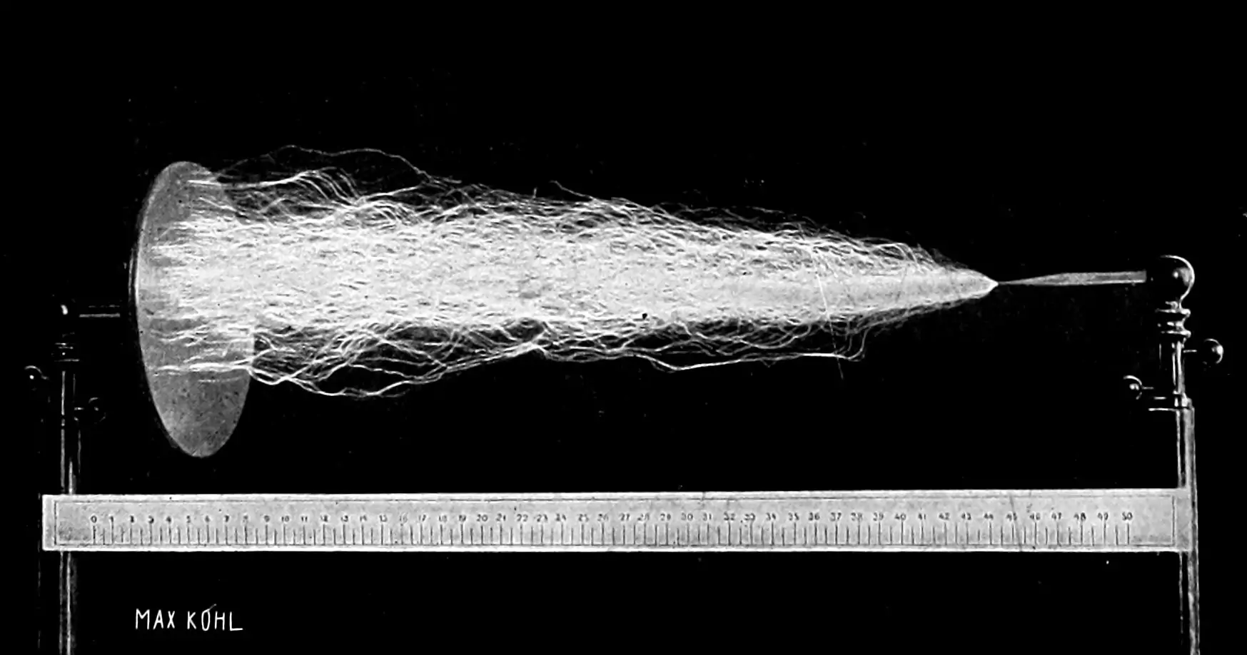
Jump processes show the difference between these. A Poisson process has paths which are not continuous with probability 1, but which are continuous in mean square and in probability.
1 Kolmogorov continuity theorem
The Kolmogorov continuity theorem gives us sufficient conditions for admitting a modification possessing a version which is Hölder of the process based on how rapidly moments of the process increments grow. Question: What gives us sufficient conditions? Lowther is good on this.
2 SDEs with rough paths
Despite the name, this is useful for smooth paths. See signatures and rough paths.
3 Connection to strong solutions of SDEs
TBD.
4 Continuity of Gaussian processes
Todo: Read Kanagawa et al. (2018) section 4, for the startling revelations:
… it is easy to show that a GP sample path \(\rv{f} \sim \mathcal{G P}(0, K)\) does not belong to the corresponding RKHS \(\mathcal{H}_{K}\) with probability 1 if \(\mathcal{H}_{K}\) is infinite dimensional… This implies that GP samples are “rougher”, or less regular, than RKHS functions … Note that this fact has been well known in the literature; see e.g., (Wahba 1990, 5) and (Lukić and Beder 2001 Corollary 7.1).
Let \(K\) be a positive definite kernel on a set \(\mathcal{X}\) and \(\mathcal{H}_{K}\) be its RKHS, and consider \(\rv{f} \sim \mathcal{G} \mathcal{P}(m, K)\) with \(m: \mathcal{X} \rightarrow \mathbb{R}\) satisfying \(m \in \mathcal{H}_{K} .\) Then if \(\mathcal{H}_{K}\) is infinite dimensional, then \(\rv{f} \in \mathcal{H}_{K}\) with probability \(0 .\) If \(\mathcal{H}_{K}\) is finite dimensional, then there is a version \(\tilde{\rv{f}}\) of \(\rv{f}\) such that \(\tilde{\rv{f}} \in \mathcal{H}_{K}\) with probability 1.
5 \(L^2\) derivatives of random fields
Robert J. Adler, Taylor, and Worsley (2016) defines \(L^2\) derivatives thus: Choose a point \(t \in \mathbb{R}^{d}\) and a sequence of \(k\) ‘directions’ \(t_{1}', \ldots, t_{k}'\) in \(\mathbb{R}^{d}\), and write these as \(t'=\left(t_{1}', \ldots, t_{k}'\right).\) From context I assume this means that these directions are supposed to have unit norm, \(\|t_j\|=1.\) We say that \(\rv{f}\) has a \(k\)-th order \(L^{2}\) partial derivative at \(t\), in the direction \(t'\), if the limit \[ D_{L^{2}}^{k} \rv{f}\left(t, t'\right) \triangleq \lim _{h_{1}, \ldots, h_{k} \rightarrow 0} \frac{1}{\prod_{j=1}^{k} h_{j}} \Delta^{k} \rv{f}\left(t, t', h\right) \] exists in mean square, where \(h=\left(h_{1}, \ldots, h_{k}\right)\). \(t_{j}\) is usually axis aligned, e.g. \(t_{j}=[\dots\, 0\, 1\,0\, \dots]^\top\). Here \(\Delta^{k} \rv{f}\left(t, t', h\right)\) is the symmetrized difference \[ \Delta^{k} \rv{f}\left(t, t', h\right)=\sum_{s \in\{0,1\}^{k}}(-1)^{k-\sum_{j=1}^{k} s_{j}} \rv{f}\left(t+\sum_{j=1}^{k} s_{j} h_{j} t_{j}'\right) \] and the limit is taken sequentially, i.e. first send \(h_{1}\to 0,\) then \(h_{2}\), etc.
That is a lot, so let us examine that for the special case of \(k=1\) and \(t_{1}=[1\,0\dots]^\top=:e_1.\) We choose a point \(t \in \mathbb{R}^{d}\) and a direction w.l.o.g. \(e_1.\) The symmetrised difference in this first order case becomes \[\begin{aligned} \Delta \rv{f}\left(t, e_1, h\right) &=\sum_{s \in\{0,1\}}(-1)^{1- s} \rv{f}\left(t+ s h_{j} e_1\right)\\ &=\rv{f}\left(t+ h_{j} e_1\right) - \rv{f}\left(t\right). \end{aligned}\] We say that \(\rv{f}\) has a first order \(L^{2}\) partial derivative at \(t\), in the direction \(e_1\), if the limit \[\begin{aligned} D_{L^{2}} \rv{f}\left(t, e_1\right) &= \lim _{h \rightarrow 0} \frac{1}{h} \Delta \rv{f}\left(t, t', h\right)\\ &= \lim _{h \rightarrow 0} \frac{\rv{f}\left(t+ h_{j} e_1\right) - \rv{f}\left(t\right)}{h} \end{aligned}\] exists in mean square. This should look like the usual first order (partial) derivative, just with the term mean-square thrown in front.
By choosing \(t^{\prime}=\left(e_{j_{1}}, \ldots, e_{j_{k}}\right)\), where \(e_{j}\) is the vector with \(j\) -th element 1 and all others zero, we can talk of the mean square partial derivatives of various orders \[ \frac{\partial^{k}}{\partial t_{j_{1}} \ldots \partial t_{j_{k}}} \rv{f}(t) \triangleq D_{L^{2}}^{k} \rv{f}\left(t,\left(e_{j_{1}}, \ldots, e_{j_{k}}\right)\right) \] of \(\rv{f}.\) Then we see that the covariance function of partial derivatives of a random field must, if it exists and is finite, be given by \[ \mathbb{E}\left\{\frac{\partial^{k} \rv{f}(s)}{\partial s_{j_{1}} \partial s_{j_{1}} \ldots \partial s_{j_{k}}} \frac{\partial^{k} \rv{f}(t)}{\partial t_{j_{1}} \partial t_{j_{1}} \ldots \partial t_{j_{k}}}\right\}=\frac{\partial^{2 k} K(s, t)}{\partial s_{j_{1}} \partial t_{j_{1}} \ldots \partial s_{j_{k}} \partial t_{j_{k}}}. \] Note that we have not assumed stationarity here, or Gaussianity, and still this process covariance function encodes a lot of information.
In the case that \(\rv{f}\) is stationary, we can use the spectral representation to analyse these derivatives. In this case, the corresponding variances have an interpretation in terms of spectral moments. We define the spectral moments \[ \omega_{j_{1} \ldots j_{N}} \triangleq \int_{\mathbb{R}^{N}} \omega_{1}^{j_{1}} \cdots \omega_{N}^{j_{N}} \nu(d \omega) \] for all multi-indices \(\left(j_{1}, \ldots, j_{N}\right)\) with \(j_{j} \geq 0\). Assuming that the underlying random field, and so the covariance function, are real valued, so that, as described above, stationarity implies that \(K(t)=K(-t)\) and \(\nu(A)=\nu(-A)\), it follows that the odd ordered spectral moments, when they exist, are zero; specifically, \[ \omega_{j_{1} \ldots j_{N}}=0 \quad \text { if } \sum_{j=1}^{N} j_{j} \text { is odd. } \]
For example, if \(\rv{f}\) has mean square partial derivatives of orders \(\alpha+\beta\) and \(\gamma+\delta\) for $, , $, \(\delta \in\{0,1,2, \ldots\}\), then \[ \begin{aligned} \mathbb{E}\left\{\frac{\partial^{\alpha+\beta} \rv{f}(t)}{\partial^{\alpha} t_{j} \partial^{\beta} t_{k}} \frac{\partial^{\gamma+\delta} \rv{f}(t)}{\partial^{\gamma} t_{\ell} \partial^{\delta} t_{m}}\right\} &=\left.(-1)^{\alpha+\beta} \frac{\partial^{\alpha+\beta+\gamma+\delta}}{\partial^{\alpha} t_{j} \partial^{\beta} t_{k} \partial^{\gamma} t_{\ell} \partial^{\delta} t_{m}} K(t)\right|_{t=0} \\ &=(-1)^{\alpha+\beta} j^{\alpha+\beta+\gamma+\delta} \int_{\mathbb{R}^{N}} \omega_{j}^{\alpha} \omega_{k}^{\beta} \omega_{\ell}^{\gamma} \omega_{m}^{\delta} \nu(d \omega). \end{aligned} \] Note that although this equation seems to have some asymmetries in the powers, these disappear due to the fact that all odd ordered spectral moments, like all odd ordered derivatives of \(K\), are identically zero.