Neural PDE operator learning
Especially forward operators. Image-to-image regression, where the images encode a physical process.
2019-10-15 — 2025-03-06
Wherein the Fourier Transform Is Employed to Learn PDE Forward-Propagators as Resolution-Agnostic Operators, and the Burgers’ Equation Is Used as a Concrete Example of One-Step Propagation Learned From Simulation Timesteps.
Neural operators are a particular way of using statistical or machine learning approaches to solve PDEs and maybe even to perform inference through them, by learning to predict some important function-to-function mapping (i.e. operator) that defines the problem. Usually this means learning the operator that predicts one step ahead from the current state .
General notes about identifying forward operators are in recursive identification, notably the pushforward trick.
1 Background
There are many function spaces and operators in this section; this could do with tidying.
Recall the setup from the ML-for-PDEs page. We are not too far from that here, i.e. the states of solutions of PDEs we are interested in are functions, mapping some spatiotemporal coordinate space \(C\) to some vector-domain \(O\). Informally, we say the state of the system is a function \(f: C\to O.\) We assume there is a function space \(\mathcal{F}\) that contains all \(f\) of interest. We might also have a forcing/boundary function \(u: C\to O'\) from a possibly different function space, \(\mathcal{U}\).
The function values for all time are given in terms of solutions in terms of differential operator \(\mathcal{D}_{\phi}\) for some parameter \(\phi\), \[\mathcal{D}_{\phi}[f]=u.\]
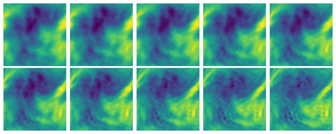
Here’s a concrete example: the Burgers’ equation \[ \begin{gathered} \partial_t f(x, t)+\partial_x\left(f^2(x, t) / 2\right)=\nu \partial_{x x} f(x, t), \quad x \in(0,1), t \in(0,1] \\ f(x, 0)=f_0(x), \quad x \in(0,1) \end{gathered} \] From this perspective \(f_0\) is a boundary condition and in fact we have sneakily introduced another one, which is that this has periodic boundary conditions on the spatial domain. In this one, \(C:= (0,1) \times (0,1].\) The internet is full of animations for the solution to this equation. Here is one:
So we could approximate that whole operator \(\mathcal{D}\). But often solving the whole thing for all time is not what we want to do because we are running our algorithm online as data comes in, or because the whole solution will not fit in RAM, or something like that.
In this setting we might think about a different operator of interest. One that ends up being useful is the PDE propagator or forward operator \(\mathcal{P}_s[f(t, \cdot;\phi)]=f( t+s, \cdot)\) which produces a representation of the entire solution surface at some future moment, given current and boundary conditions, and some parameters \(\phi\). The forward propagator is what most methods on this page target.
Learning a PDE operator is naturally expressed by a layer which acts on functions and is indifferent to how those functions are discretised, in particular the scale at which they are discretised. We learn to approximate \(\mathcal{P}_s[ f(t, \cdot); \phi]\) from data by minimising prediction error over input/output pairs \(\left\{a_{j}, u_{j}\right\}_{j=1}^{N}\) where \(a_{j}\in \mathscr{A}\) and \(u_{j}=\mathcal{P}^{\dagger}_{1,\theta}(a_{j})+\epsilon_{j}\) where \(\epsilon_{j}\) is a corrupting noise. Further, we observe these functions only at certain points \(\{x_{1},\dots,x_{n}\}\subset D.\) We approximate \(\mathcal{P}^{\dagger}_{1,\phi,\theta}\) by choosing good parameters \(\theta^{\dagger} \in \Theta\) from the parameter space in some parametric family of maps \(\{\mathcal{P}^{\dagger}_{1,\phi,\theta}\left(\cdot, \right);\theta\in\Theta\}\) so that \(\mathcal{P}^{\dagger}_{1,\theta,\phi^{\dagger}}\left(\cdot, \right)=\approx \mathcal{P}^{\dagger}_{1,\phi}\). Specifically, we minimise some cost functional \(C: \mathscr{U} \times \mathscr{U} \rightarrow \mathbb{R}\) in the hope that we are solving \[ \min _{\theta \in \Theta} \mathbb{E}_{a \sim \mu}\left[C\left(\mathcal{P}_{1,\phi}(a), \mathcal{P}^{\dagger}_{1,\phi,\theta}(a)\right)\right]. \]
2 Fourier neural operator
I’ve done a lot of things with the Fourier Neural Operator family. Too many things, in fact, to blog here; as such this section is out of date.
Zongyi Li blogs a neat trick: We use Fourier transforms to capture resolution-invariant and non-local behaviour in PDE forward-propagators. Essentially, we learn to approximate \(\mathcal{P}_1: \mathscr{A}\to\mathscr{A}.\) There is a bouquet of papers designed to leverage the trick (Li, Kovachki, Azizzadenesheli, Liu, Bhattacharya, et al. 2020b, 2020a; Li, Kovachki, Azizzadenesheli, Liu, Stuart, et al. 2020). See also Anima Anandkumar’s presentation, which phrases this in terms of Green’s functions and their relationship with Fourier transforms. See also nostalgebraist who has added some interesting commentary and also fixed up a typo in this page for me (Thanks!). Yannic Kilcher’s Fourier Neural Operator for Parametric Partial Differential Equations Explained is popular but I have not watched it. Code was at zongyi-li/fourier_neural_operator. Now generalised and professionalised at Neural Operators in PyTorch.
In most common applications, Fourier Neural Operator is a method for approximating \(\mathcal{P}_{1,\phi}\).
Ok, so what is going on?
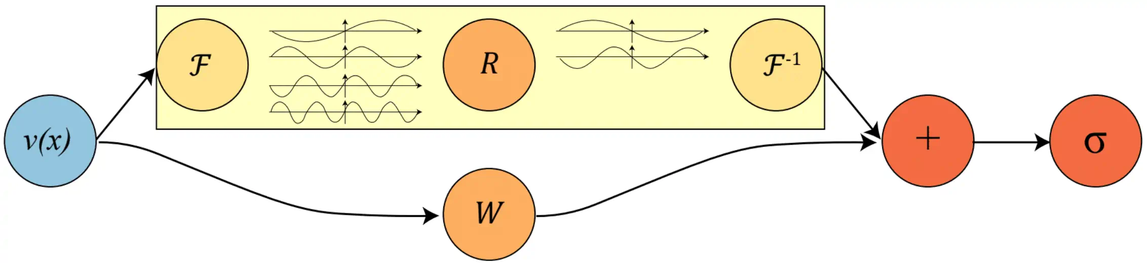
For the neural Fourier operator in particular we assume that \(\mathcal{\mathcal{G}}_{\phi}\) has a particular iterative form, i.e. \(\mathcal{G}= Q \circ V_{T} \circ V_{T-1} \circ \ldots \circ V_{1} \circ P\). We introduce a new space \(\mathscr{V}=\mathscr{V}\left(D ; \mathbb{R}^{d_{v}}\right)\). \(P\) is a map \(\mathscr{A}\to\mathscr{V}\) and \(Q\) is a map \(\mathscr{V}\to\$\mathscr{U}\), and each \(V_{t}\) is a map \(\mathscr{V}\to\mathscr{V}\). Each of \(P\) and \(Q\) is ‘local’ in that they depend only upon pointwise evaluations of the function, e.g. for \(a\in\mathscr{A}\), \((Pa)(x)=p(a(x))\) for some \(p:\mathbb{R}^{d_{a}}\to\mathbb{R}^{d_{v}}\). Each \(v_{j}\) is function \(\mathbb{R}^{d_{v}}\). As a rule we are assuming \(d_{v}>d_{a}>d_{u}.\) \(V_{t}\) is not local. In fact, we define \[ (V_{t}v)(x):=\sigma\left(W v(x)+\left(\mathcal{K}(a ; \phi) v\right)(x)\right), \quad \forall x \in D \] where \(\mathcal{K}(\cdot;\phi): \mathscr{A} \rightarrow \mathcal{L}\left(\mathscr{V}, \mathscr{V}\right)\). This map is parameterized by \(\phi \in \Theta_{\mathcal{K}}\). \(W: \mathbb{R}^{d_{v}} \rightarrow \mathbb{R}^{d_{v}}\) is a linear transformation, and \(\sigma: \mathbb{R} \rightarrow \mathbb{R}\) is a local, component-wise, non-linear activation function. \(\mathcal{K}(a ; \phi)\) is a kernel integral transformation, by which is meant \[ \left(\mathcal{K}(a ; \phi) v\right)(x):=\int_{D} \kappa_{\phi}(x, a(x), y, a(y)) v(y) \mathrm{d} y, \quad \forall x \in D \] where \(\kappa_{\phi}: \mathbb{R}^{2\left(d+d_{a}\right)} \rightarrow \mathbb{R}^{d_{v} \times d_{v}}\) is some mapping parameterized by \(\phi \in \Theta_{\mathcal{K}}\).
Anyway, it looks like this:
Because this is neural net land we can be a certain type of sloppy and we don’t worry overmuch about the bandwidth of the signals we approximate; We keep some small number of low harmonics from the Fourier transform and use fairly arbitrary non-Fourier maps too, and conduct the whole thing in a “high” dimensional space with vague relationship to the original problem without worrying too much about what it means.
See Kovachki, Lanthaler, and Mishra (2021) for some analysis of the performance of this method.
2.1 Justification in terms of Fourier transform
The basic concept is heuristic and the main trick is doing lots of accounting of dimensions, and being ok with an arbitrary-dimensional Fourier transform \(\mathcal{F}:(D \rightarrow \mathbb{R}^{d}) \to (D \rightarrow \mathbb{C}^{d})\), which looks like this:
\[\begin{aligned} (\mathcal{F} f)_{j}(k) &=\int_{D} f_{j}(x) e^{-2 i \pi\langle x, k\rangle} \mathrm{d} x \\ \left(\mathcal{F}^{-1} f\right)_{j}(x) &=\int_{D} f_{j}(k) e^{2 i \pi\langle x, k\rangle} \mathrm{d} k \end{aligned}\] for each dimension \(j=1, \ldots, d\).
We notionally use the property that convolutions become multiplications under Fourier transform, which motivates the use of convolutions to construct our operators. Good.
2.2 Justification in terms of Green’s functions
Now what if \(\mathcal{D}\) is linear? Then we can write solutions in terms of convolutions of Green’s functions: \[ \begin{aligned} -\nabla \cdot(a(x) \nabla u(x)) & =f(x), & & x \in D \\ u(x) & =0, & & x \in \partial D \end{aligned} \] Inverse of differential operator can be written in form of kernel: \[ u(x)=\int_D G_a(x, y) f(y) d y \] Where \(\mathrm{G}\) is the Green’s function (+ a correction term for non-zero boundaries)
To my mind, this is very similar to the Fourier transform justification, but in a different language, because we can convolve functions by their Fourier transforms; see above.
We immediately throw out the dependence on \(a\) in the kernel definition, replacing it with \[\kappa_{\phi}(x, a(x), y, a(y)) := \kappa_{R}(x-y)\] so that the integral operator becomes a convolution. This convolution can be calculated cheaply in Fourier space, which suggests we may as well define and calculate it also in Fourier space. Accordingly, the real work happens when they define the Fourier integral operator: \[ \left(\mathcal{K}(\phi) v\right)(x)=\mathcal{F}^{-1}\left(R \cdot\left(\mathcal{F} v\right)\right)(x) \quad \forall x \in D \] where $R $ is the Fourier transform of a periodic function \(\kappa: D \rightarrow \mathbb{R}^{d_{v} \times d_{v}}\) parameterized by \(\phi \in \Theta_{\mathcal{K}}\). Checking our units, we have that \(\left(\mathcal{F} v\right):D \to \mathbb{C}^{d_{v}}\) and \(R (k): D \to \mathbb{C}^{d_{v} \times d_{v}}\). In practice, since we can work with a Fourier series rather than a continuous transform, we will choose \(k\in\{0,1,2,\dots,k_{\text{max}}\}\) and then $R $ can be represented by a tensor \(\mathbb{C}^{k_{\text{max}}\times d_{v}\times d_{v}}.\) 1 Not quite sure who is right. Caveat emptor. We can use a different \(W\) and \(R\) for each iteration if we want, say \(\{W_t,R_t\}_{1\leq t \leq T}\). So, the parameters of each of these, plus those of the maps \(P,Q\) comprise the parameters of the whole process.
Anyway, every step in this construction is differentiable in those parameters, and some of the steps can even be found rapidly using FFTs and so on, so we are done with the setup, and have an operator that can be learned from data.
2.3 Pros
Is this method any good? Yes. In the happy but very specific world where the PDE solutions are not too far from periodic, this model converges fast to an excellent approximation of the classical numerical solution, at a very low cost (Takamoto et al. 2022). Surprisingly (to me) it is also a really good estimator of the Jacobian of the solution (MacKinlay et al. 2021). This is not magic — we still need to train the models — but even the cost of that is remarkably low, especially if we train over a fixed data set.
The question is: how do we handle things outside that very specific world?
2.4 Cons
Quibble: They use the term ‘resolution-invariant’ loosely at a few points in the paper, and it takes some work to understand the actual defensible claim. They do not actually prove that things are resolution invariant per se. Rather, it is not even clear what that would specifically mean in this context — there is no attempt to prove Nyquist conditions or other sampling-theoretic properties over the spatial domain. And, AFAICT in the time domain their method is resolution-dependent in every sense. Step size is fixed.
What is clear and what I think they mean is that there is an obvious interpretation of the solution as a continuous operator, in the sense that it can be evaluated at arbitrary (spatial) points for the same computational cost as evaluating it at the training points. Thus there is a sense in which it does not depend upon the resolution of the training set, in that we don’t need any resampling of the solution to evaluate the functions our operator produces at unobserved coordinates.
What does this get us? You can, in a certain sense, treat many network structures as discrete approximations to PDE operators with a certain resolution (at least, deep Resnets with ReLU activations have such an interpretation, presumably others) and then use resampling methods to evaluate them at a different resolution, which is a more laborious process that potentially gets a similar result — see the notebook on deep learning as dynamical system for examples of doing that.
Next quibble: Why Fourier transforms, instead of a different basis? Their rationale is that integral operators can be understood as continuous convolutions in the linear case, and therefore a bit like convolutions more generally. Heuristically, stacked continuous convolutions and non-linearities might well-approximate the operations of solving a nonlinear PDE. So convolutions are what we want, and Fourier transforms turn convolutions into multiplications so we can use them. It might sound like we should use actual convolutional neural networks to solve the PDE, but that would impose a given resolution on the solution which is not what we want. For me, a better rationale is that this Fourier transform puts us in a “nice” basis for PDEs because Fourier transforms have well-understood interpretations which encode derivatives, translations, interpolations and other useful operations, which is why we use them in classic PDE solvers. The convolution thing is more “deep net-like” though.
Also Fourier transforms are notionally fast, which is another popular deep net rationale. Implementation detail: the authors do not make any particular effort to be maximally fast by using dilation to truncate the Fourier series. Instead they calculate the whole Fourier transform then throw some bits out. Presumably because they were already fast enough without bothering with being clever.
OTOH Fourier series also encode some troubling assumptions. Essentially these amount to an assumption that the basis functions are periodic, which in turn amounts to assuming that the domain of functions is toroidal, or, I suppose, a box with uniform boundary conditions. This is pretty common, but also annoying. Li, Kovachki, Azizzadenesheli, Liu, Bhattacharya, et al. (2020b) argue that does not matter because the edge effects can be more-or-less ignored and that things will still work OK because of the “local linear projection” part, which is … fine I guess? Maybe true. It still grates. Certainly the boundary conditions situation will just be messy AFAICT for any neural operator so I am at ease with the idea they would like to simply ignore it for now.
Would alternative bases fix that boundary problem, or just be more of an annoying PITA? Spherical neural operators (Bonev et al. 2023; Mahesh et al. 2024) are now a thing, and much more sane for applications on nearly-spherical domains, such as the Earth’s surface.
Would there be anything to gain from learning a basis for the expansion? DeepONet is a related method that learns bases. Certainly you would lose speed.
The FNO method uses a lot of the right buzzwords to sound like a kernel trick approach, and one can’t help but feel there might be a logical Gaussian process regression formulation with nice Bayesian interpretation. I suppose it could possibly be approximated as ‘just’ another deep Gaussian process with some tactical assumptions, perhaps infinite-width asymptotics. Laplace approximation? Or a variational approximation?
2.5 Is FNO secretly a DeepONet?
Kinda sorta. See Kovachki, Lanthaler, and Mishra (2021), Lu et al. (2022).
2.6 Avoiding inverse transform
Poli et al. (2022) transforms once (how DO they recover the original domain? not obvious from skimming) rather than transforming inverse transforming. This is notionally faster.
2.7 Boundary conditions
Are hard to handle in FNOs. Many papers mention possible solutions. X. Liu, Yeo, and Lu (2020) just assumes that there are some initial conditions and boundaries can be “handled” by hoping that simulating a toroidal domain then cutting out a segment of interest. Possibly alternative transforms would help.
3 U-net
TBD.
4 Active learning
Seems logical. But how much of that is there? Gajjar, Hegde, and Musco (2022).
5 Alternative basis transforms in spectral operators
The Fourier transform is generalised to the Laplace transform in Q. Cao, Goswami, and Karniadakis (2023).
Alternative transforms are important in the DeepONet lineages.
Learnable transforms are discussed in Meuris, Qadeer, and Stinis (2023); Witman et al. (2022).
6 DeepONet
From the people who brought us the PINN, comes Lu, Jin, and Karniadakis (2020). The setup is related to the PINNs, but AFAICT differs in a few ways in that
- we don’t (necessarily?) use the derivative information at the sensor locations
- we learn an operator mapping initial/latent conditions to output functions
- we decompose the input function space into a basis and then sample from the bases in order to span (in some sense) the input space at training time
The authors argue they have found a good topology for a network that does this and efficiently solves PDEs
A DeepONet consists of two sub-networks, one for encoding the input function at a fixed number of sensors \(x_i, i = 1, \dots, m\) (branch net), and another for encoding the locations for the output functions (trunk net).
This addresses some problems with generalisation that make the PINN setup seem unsatisfactory; in particular we can change the inputs, or project arbitrary inputs forward.
The boundary conditions and input points appear to stay fixed though, and inference of the unknowns is still vexed.
Implementations?
Ceyron/trainax: Training methodologies for autoregressive neural operators in JAX.
pytorch via TorchPhysics
tensorflow
🚧TODO🚧
7 Recursive estimation
See recursive identification for generic theory of learning under the distribution shift induced by a moving parameter vector.
8 Conservation-laws-ey-architectures
Lanthaler and Stuart (2023):
Neural operator architectures employ neural networks to approximate operators mapping between Banach spaces of functions; they may be used to accelerate model evaluations via emulation, or to discover models from data. Consequently, the methodology has received increasing attention over recent years, giving rise to the rapidly growing field of operator learning. The first contribution of this paper is to prove that for general classes of operators which are characterized only by their \(C^r\)- or Lipschitz-regularity, operator learning suffers from a “curse of parametric complexity”, which is an infinite-dimensional analogue of the well-known curse of dimensionality encountered in high-dimensional approximation problems. The result is applicable to a wide variety of existing neural operators, including PCA-Net, DeepONet and the FNO. The second contribution of the paper is to prove that this general curse can be overcome for solution operators defined by the Hamilton-Jacobi equation; this is achieved by leveraging additional structure in the underlying solution operator, going beyond regularity. To this end, a novel neural operator architecture is introduced, termed HJ-Net, which explicitly takes into account characteristic information of the underlying Hamiltonian system. Error and complexity estimates are derived for HJ-Net which show that this architecture can provably beat the curse of parametric complexity related to the infinite-dimensional input and output function spaces.
Ruhe et al. (2023),Brandstetter et al. (2022):
Partial differential equations (PDEs) see widespread use in sciences and engineering to describe simulation of physical processes as scalar and vector fields interacting and coevolving over time. Due to the computationally expensive nature of their standard solution methods, neural PDE surrogates have become an active research topic to accelerate these simulations. However, current methods do not explicitly take into account the relationship between different fields and their internal components, which are often correlated. Viewing the time evolution of such correlated fields through the lens of multivector fields allows us to overcome these limitations. Multivector fields consist of scalar, vector, as well as higher-order components, such as bivectors and trivectors. Their algebraic properties, such as multiplication, addition and other arithmetic operations can be described by Clifford algebras. To our knowledge, this paper presents the first usage of such multivector representations together with Clifford convolutions and Clifford Fourier transforms in the context of deep learning. The resulting Clifford neural layers are universally applicable and will find direct use in the areas of fluid dynamics, weather forecasting, and the modeling of physical systems in general. We empirically evaluate the benefit of Clifford neural layers by replacing convolution and Fourier operations in common neural PDE surrogates by their Clifford counterparts on 2D Navier-Stokes and weather modeling tasks, as well as 3D Maxwell equations. For similar parameter count, Clifford neural layers consistently improve generalization capabilities of the tested neural PDE surrogates.
9 Pseudo-physics
I just saw this neat idea get knocked back for ICLR: Chen et al. (2024):
Recent advancements in operator learning are transforming the landscape of computational physics and engineering, especially alongside the rapidly evolving field of physics-informed machine learning. The convergence of these areas offers exciting opportunities for innovative research and applications. However, merging these two realms often demands deep expertise and explicit knowledge of physical systems, which may be challenging or even impractical in relatively complex applications. To address this limitation, we propose a novel framework: Pseudo Physics-Informed Neural Operator (PPI-NO). In this framework, we construct a surrogate physics system for the target system using partial differential equations (PDEs) derived from simple, rudimentary physics knowledge, such as basic differential operators. We then couple the surrogate system with the neural operator model, utilizing an alternating update and learning process to iteratively enhance the model’s predictive power. While the physics derived via PPI-NO may not mirror the ground-truth underlying physical laws — hence the term “pseudo physics” — this approach significantly enhances the accuracy of current operator learning models, particularly in data scarce scenarios. Through extensive evaluations across five benchmark operator learning tasks and an application in fatigue modeling, PPI-NO consistently outperforms competing methods by a significant margin. The success of PPI-NO may introduce a new paradigm in physics-informed machine learning, one that requires minimal physics knowledge and opens the door to broader applications in data-driven physics learning and simulations.
This is kind of neat IMO; it formalises a trick used in the FNO, which implicitly makes derivatives available to the network by using a Fourier transform, but in a more general way.
10 Complexity of neural operators
(Boullé, Halikias, and Townsend 2023; Lanthaler and Stuart 2023)
11 Using KANs
Kolmogorov-Arnold Neural Networks are a way of learning operators that are more interpretable than MLPs, and potentially more expressive. Might help with operator learning? (Abueidda, Pantidis, and Mobasher 2024; Howard et al. 2024; Koenig, Kim, and Deng 2024; Z. Liu et al. 2024; Y. Wang et al. 2024; Kunpeng Xu, Chen, and Wang 2024)
12 On intersting geometries
Challenging. See operator learning on interesting geometries.
13 Incoming
Ilze Amanda Auzina’s tutorial DNN Tutorial 2 Part II: Physics inspired Machine Learning for Phillip Lippe’s Deep Learning course at the University of Amsterdam. * pyg-team/pytorch_geometric: Graph Neural Network Library for PyTorch * Peter Woit, Symmetry and Physics
It’s getting late, but I can’t help myself. Reading too many wrong things about symmetry and physics on Twitter has forced me to do this. And, John Baez says I don’t explain things. So, here’s what the relationship between symmetry and physics really is.
-
We introduce Learning controllable Adaptive simulation for Multi-resolution Physics (LAMP), the first fully DL-based surrogate model that jointly learns the evolution model, and optimizes spatial resolutions to reduce computational cost, learned via reinforcement learning. We demonstrate that LAMP is able to adaptively trade-off computation to improve long-term prediction error, by performing spatial refinement and coarsening of the mesh. LAMP outperforms state-of-the-art (SOTA) deep learning surrogate models, with an average of 33.7% error reduction for 1D nonlinear PDEs, and outperforms SOTA MeshGraphNets + Adaptive Mesh Refinement in 2D mesh-based simulations.
14 References
Footnotes
NB — my calculations occasionally came out differing from the versions the authors gave in the paper with regards to the dimensionality of the spaces.↩︎