Normalising flows

1 Basic

AFAICT the terminology is chosen to imply that the reparameterization should be differentiable, bijective and computationally convenient Ingmar Shuster’s summary of the foundational (Rezende and Mohamed 2015) is a little snarky:

The paper adopts the term normalising flow for referring to the plain old change of variables formula for integrals.

I have had the dissertation (Papamakarios 2019) recommended to me a lot as a summary for this field, although I have not read it. The shorter summary paper looks good though (Papamakarios et al. 2021). See Kobyzev, Prince, and Brubaker (2021) for a recent review.

Normalizing flows are a method of variational inference. As with typical variational inference, it is convenient for us while doing inference to have a way of handling an approximate posterior density over the latent variables $\mathsf{z}$ given the data $\mathsf{x}$. The real posterior density $p(z|x)$ is intractable, so we construct an approximate density $q_{\varphi }(z|x)$ parameterised by some variational parameters $\varphi$. We have certain desiderata. Specifically, we would like to efficiently…

1. calculate the density $q_{\varphi }(z|x)$, such that…
2. we can estimate expectations/integrals with respect to $q_{\varphi }(\cdot |z)$ in the sense that we can estimate $\int q_{\varphi }(\cdot |z)f(z)\mathrm{d}z,$ which we are satisfied to do via Monte Carlo, and so it will suffice if we can simulate from this density, and
3. we can differentiate through this density with respect to the variational parameters to find $\frac{\partial }{\partial \varphi }{q}_{\varphi }(z|x).$
4. Our method is ‘flexible enough’ to approximate a complicated, messy posterior density.

The whole problem in such a case would entail solving for the variational objective:

$$\begin{array}{rl}\log p_{\theta }\left(x\right)& \ge \mathcal{L}(\theta ,\varphi ;x)\\ & ={\mathbb{E}}_{q_{\varphi }(z|x)}[-\log q_{\varphi }(z|x)+\log p_{\theta }(x,z)]\\ & =-\mathrm{KL}(q_{\varphi }(z|x)\parallel p_{\theta }(z))+{\mathbb{E}}_{q_{\varphi }(z|x)}[\log p_{\theta }(x|z)]\\ & =-\mathcal{F}(\theta ,\varphi )\end{array}$$

Here $p_{\theta }(x)$ is the marginal likelihood of the generative model for the data, $p_{\theta }(x|z)$ the density of observations given the latent factors and $\theta$ parameterises the density of the generative model.

(For the next bit, we temporarily suppress the dependence on $\mathsf{x}$ to avoid repetition, and the dependence of the transforms and density upon $\varphi$.)

Normalizing flows use the reparameterization trick as an answer to those desiderata. Specifically, we assume that for some function (not density!) $f:{\mathbb{R}}^D\to {\mathbb{R}}^D,$ that $$\mathsf{z}=f({\mathsf{z}}_0)$$ and that ${\mathsf{z}}_0\sim q_0=\mathcal{N}(0,\mathrm{I})$ (or some similarly easy distribution). It turns out that by imposing some extra restrictions, we can do most of the heavy lifting in this algorithm through this simple ${\mathsf{z}}_0\sim q_0$ and still get the power of a fancy posterior $\mathsf{z}\sim q.$

Now we can calculate (sufficiently nice) expectations with respect to $\mathsf{z}$ using the law of the unconscious statistician $$\mathbb{E}f(\mathsf{z})=\int f(z)q_0(z)\mathrm{d}z.$$

However, we need to impose additional conditions to guarantee a tractable form for the densities; in particular we impose the restriction that $f$ is invertible, so that we can use the change of variables formula to find the density

$$q\left(z\right)=q_0(f^{-1}(z))\left|\det \frac{\partial f^{-1}(z)}{\partial z}\right|=q_0(f^{-1}(z)){\left|\det \frac{\partial f(z)}{\partial z}\right|}^{-1}.$$

We can economise on function inversions since we are evaluating always via simulating $\mathsf{z}$ from $f({\mathsf{z}}_0)$, i.e. $\mathsf{z}:=f({\mathsf{z}}_0)$, so we can write

$$q\left(\mathsf{z}\right)=q_0({\mathsf{z}}_0){\left|\det \frac{\partial f(\mathsf{z})}{\partial \mathsf{z}}\right|}^{-1}.$$

We do not need, that is to say, $f$ inversions, just the Jacobian determinant, which might be easier. Spoiler: later on we construct some $f$ transforms for which it is easy-ish to find that Jacobian determinant without inverting the function.

We want this mapping to depend upon $\mathsf{x}$ and the parameters $\varphi$ so we reintroduce that dependence now. We parameterize these functions $f_{\varphi }(\mathsf{z}):=f(\mathsf{z},\varphi (\mathsf{x}));$ that is, our $\varphi$ parameters are a learned mapping from observation ${\mathsf{z}}_0$ to a posterior sample from the latent variable $\mathsf{z}$ with density $q_K(z_K|x)\simeq p_{\theta }(z|x)$ such that, if we configure everything just right, $q_K(z_K|x)\simeq p_{\theta }(z|x)$.

And indeed it is not too hard to find a recipe for optimising these parameters. We may estimate the following derivatives $_{} ( x ) $ and ${\mathrm{\nabla }}_{\varphi }\mathcal{F}(x)$ which is sufficient to minimise $\mathcal{F}(\theta ,\varphi )$ by gradient descent.

In practice we are doing this in a big data context, so we use stochastic subsamples from $x$ to estimate the gradient and Monte Carlo simulations from ${\mathsf{z}}_0$ to estimate the necessary integrals with respect to $q_K(\cdot |\mathsf{x}).$

So far so good. But it turns out that this is not in general very tractable, because determinants are notoriously expensive to calculate, scaling poorly — $\mathcal{O}(D^3)$ — in the number of dimensions, which we expect to be large in trendy neural-network-type problems.

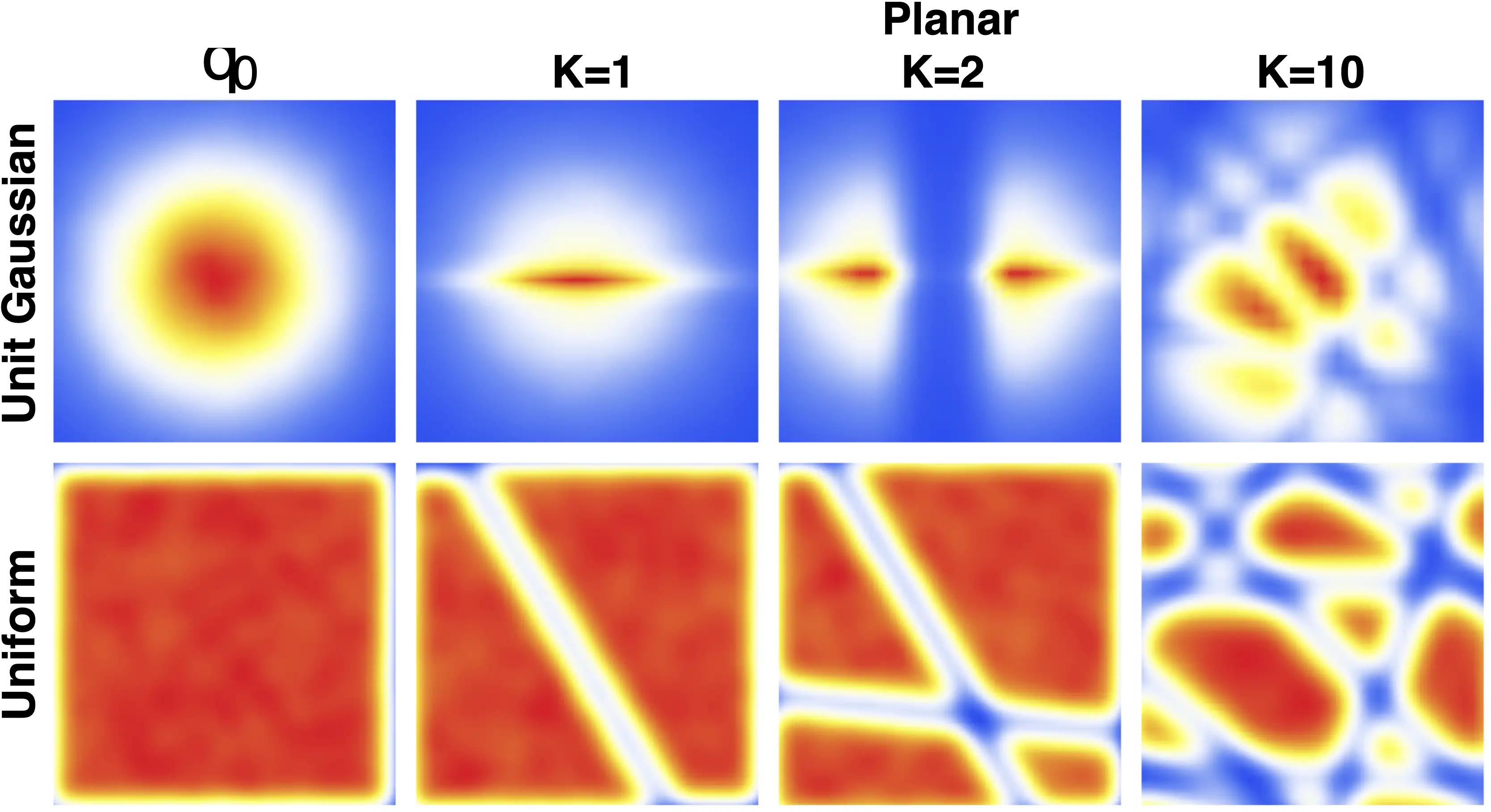
We look for restrictions on the form of $f_{\varphi }$ such that $\det \frac{\partial f_{\varphi }}{\partial z}$ is cheap and yet the approximate $q$ they induce is still “flexible enough”. The normalizing flow solution is to choose compositions of some class of cheap functions $${\mathsf{z}}_K=f_K\circ \dots \circ f_2\circ f_1\left({\mathsf{z}}_0\right)\sim q_K.$$

By induction on the change of variables formula (and using the logarithm for tidiness), we can find the density of the variable mapped through this flow as

$$\log q_K({\mathsf{z}}_K|x)=\log q_0({\mathsf{z}}_0|x)-\sum _{k=1}^K\log \left|\det \left(\frac{\partial f_k\left({\mathsf{z}}_{k-1}\right)}{\partial {\mathsf{z}}_{k-1}}\right)\right|$$

Compositions of such cheap functions should also be cheap-ish and each iteration would add extra flexibility.

But which $f_k$ mappings are cheap? The archetypal one from (Rezende and Mohamed 2015) is the “planar flow”:

$$f(\mathsf{z})=\mathsf{z}+uh(w^{\mathrm{\top }}\mathsf{z}+b)$$ where $ u, w ^{D}, b $ and $h:\mathbb{R}\to \mathbb{R}$ is some monotonic differentiable activation function.

There is a standard identity, the matrix determinant lemma $\det (\mathrm{I}+u{v}^{\mathrm{\top }})=1+u^{\mathrm{\top }}v,$ from which it follows that $$\begin{array}{rl}\det \frac{\partial f}{\partial z}& =\det (\mathrm{I}+u{h}^{\prime }(w^{\mathrm{\top }}z+b)w^{\mathrm{\top }})\\ & =1+u^{\mathrm{\top }}{h}^{\prime }(w^{\mathrm{\top }}z+b)w.\end{array}$$ We can often simply parameterise acceptable domains for functions like these so that they remain invertible; For example if $h\equiv \tanh$ a sufficient condition is $u^{\mathrm{\top }}w\ge 1.$ This means that we know it should be simple to parameterise these weights $u,w,b$. Or, as in our application, that it is easy to construct functions $\varphi :x\mapsto u,w,b$ which are guaranteed to remain in an invertible domain.

For functions like this, the determinant calculation is cheap, and does not depend at all on the ambient dimension of $\mathsf{x}$. However, we might find it hard to persuade ourselves that this mapping is flexible enough to represent $q$ well, at least without letting $K$ be large, as the mapping must pass through a univariate “bottleneck” $w^{\mathrm{\top }}\mathsf{z}.$ Indeed, empirically this mapping does not in fact perform well and a lot of time has been spent trying to do better.

The parallel with the problem of finding covariance kernels is interesting. In both cases we have some large function class we wish to parameterise so we can search over it, but we restrict it to a subset with computationally convenient properties and a simple domain.

2 A fancier flow

There are various solutions to this problem; an illustrative one is Sylvester flow (van den Berg et al. 2018) which, instead of the matrix determinant lemma uses a generalisation, Sylvester’s determinant identity. This tells us that for all $\mathrm{A}\in {\mathbb{R}}^{D\times M},\mathrm{B}\in {\mathbb{R}}^{M\times R}$, $$\det ({\mathrm{I}}_D+\mathrm{A}\mathrm{B})=\det ({\mathrm{I}}_M+\mathrm{B}\mathrm{A})$$ where $ {M}$ and $ {D}$ are respectively $M $ and $ D$ dimensional identity matrices.

This suggests we might exploit a generalized planar flow, $$f(\mathsf{z}):=\mathsf{z}+\mathrm{A}h(\mathrm{B}\mathsf{z}+b)$$ with $ ^{D M}, ^{M D}, b ^{M},$ and $M\le D.$ The determinant calculation scales as $\mathcal{O}(M^3)\ll \mathcal{O}(D^3),$ which is cheap-ish and, we hope, gives us enough additional scope to design sufficiently flexible flows. $M\ge 1$ is a bottleneck parameter.

The price is an additional parameterisation problem. How do we select $\mathrm{A}$ and $\mathrm{B}$ such that they are still invertible for a given $h$? The solution in (van den Berg et al. 2018) is to break this into two simpler parameterisation problems.

They choose $f(\mathsf{z}):=\mathsf{z}+\mathrm{Q}\mathrm{R}h(\tilde{\mathrm{R}}{\mathrm{Q}}^T\mathsf{z}+\mathrm{b})$ where $\mathrm{R}$ and $\tilde{\mathrm{R}}$ are upper triangular $M\times M$ matrices, and $Q$ is a $D\times M$ matrix with orthonormal columns $\mathrm{Q}=({\mathrm{q}}_1\dots {\mathrm{q}}_M).$ Using the Sylvester identity on this $f$ we find

$$\det \frac{\partial f}{\partial z}=\det ({\mathrm{I}}_M+\mathrm{diag}\left(h^{\prime }(\tilde{\mathrm{R}}{\mathrm{Q}}^{T}z+b)\right)\tilde{\mathrm{R}}\mathrm{R})$$

They also show that if, in addition,

1. $h:\mathbb{R}⟶\mathbb{R}$ is a smooth function with bounded, positive derivative and
2. if the diagonal entries of $\mathrm{R}$ and $\tilde{\mathrm{R}}$ satisfy $r_{ii}{\tilde{r}}_{ii}>-1/{\Vert h^{\prime }\Vert }_{\mathrm{\infty }}$ and
3. $\tilde{\mathrm{R}}$ is invertible,

then $f$ is invertible as required.

Now all we need to do is choose a differentiable parameterisation of the upper-triangular $\mathrm{R},$ the upper-triangular invertible $\tilde{\mathrm{R}}$ with appropriate diagonal entries and the orthonormal matrix, $Q$. That is a whole other story though.

3 Spline

The type of flow that everyone seems to use in practice for moderate dimensionality is the spline flow (Durkan et al. 2019).

4 Glow

Generative flow for images and similar stuff (Durk P. Kingma and Dhariwal 2018).

5 For density estimation

I am no longer sure what distinction I wished to draw with this heading, but see (Esteban G. Tabak and Vanden-Eijnden 2010; E. G. Tabak and Turner 2013) and maybe also check out transport maps.

🏗

6 Tutorials

• Rui Shu explains change of variables in probability and shows how it induces the normalizing flow idea, which the reparameterisation trick forms part of.
• PyMC3 example of a non-trivial usage.
• Adam Kosiorek summarises some fancy variants of normalising flow.
• Eric Jang did a tutorial which explains how this works in Tensorflow.
• Praveen on Ruiz, Titsias, and Blei (2016).
• Dustin Tran, Denoising Criterion for Variational Auto-Encoding Framework
• Shakir Mohamed, Machine Learning Trick of the Day (4): Reparameterisation Tricks
• Papamakarios et al. (2021)
• Eric Jang on normalising flows

7 General measure transport

See transport maps.

8 Representational power of

A CMU team argues

The most fundamental restriction of the normalising flow paradigm is that each layer needs to be invertible. We ask whether this restriction has any ‘cost’ in terms of the size, and in particular the depth, of the model. Here we’re counting depth in terms of the number of the invertible transformations that make up the flow. A requirement for large depth would explain training difficulties due to exploding (or vanishing) gradients. Since the Jacobian of a composition of functions is the product of the Jacobians of the functions being composed, the min (max) singular value of the Jacobian of the composition is the product of the min (max) singular value of the Jacobians of the functions. This implies that the smallest (largest) singular value of the Jacobian will get exponentially smaller (larger) with the number of compositions.

A natural way of formalising this question is by exhibiting a distribution which is easy to model for an unconstrained generator network but hard for a shallow normalising flow. Precisely, we ask: is there a probability distribution that can be represented by a shallow generator with a small number of parameters that could not be approximately represented by a shallow composition of invertible transformations?

We demonstrate that such a distribution exists.

…To reiterate the takeaway: a GLOW-style linear layer in between affine couplings could in theory make your network between 5 and 47 times smaller while representing the same function. We now have a precise understanding of the value of that architectural choice!

9 Conditioned

(Koehler, Mehta, and Risteski 2020; Winkler et al. 2023) TBC

10 Implementations

• probabilists/zuko: Normalising flows in PyTorch — Seems active

• Numpyro includes normalising flows

  • Documentation

• Pyro includes normalising flows, albeit not especially fancy ones:

  • example
  • API documentation

• flowtorch / Source (Formerly Meta-backed, I think now independent?)

• VincentStimper/normalising-flows

11 References