Efficient Langevin sampling Gaussian distributions

1 Problem Setting

We aim to sample from a multivariate Gaussian distribution:

$$\mathbf{x}\sim \mathcal{N}(\mathit{\mu },\mathrm{\Sigma })$$

where:

• $\mathit{\mu }\in {\mathbb{R}}^D$ is the known mean vector.
• $\mathrm{\Sigma }\in {\mathbb{R}}^{D\times D}$ is the notional known covariance matrix, which might be too large to actually compute, let alone factorise for sampling in the usual way.

2 Langevin Dynamics for Sampling

Langevin dynamics provide a way to sample from a target distribution by simulating a stochastic differential equation (SDE) whose stationary distribution is the desired distribution. For a Gaussian distribution, the SDE simplifies due to the properties of the normal distribution (i.e. Gaussians all the way down).

The continuous-time Langevin equation is

$$d{\mathbf{x}}_t=-\mathrm{\nabla }U({\mathbf{x}}_t)dt+\sqrt{2}d{\mathbf{W}}_t$$

where

• $U(\mathbf{x})$ is the potential function related to the target distribution $p(\mathbf{x})$ via $p(\mathbf{x})\propto e^{-U(\mathbf{x})}$.
• $d{\mathbf{W}}_t$ represents the increment of a Wiener process (standard Brownian motion).

For our Gaussian distribution, the potential function is:

$$U(\mathbf{x})=\frac{1}{2}(\mathbf{x}-\mathit{\mu }{)}^{\mathrm{\top }}{\mathrm{\Sigma }}^{-1}(\mathbf{x}-\mathit{\mu })$$

We discretize the Langevin equation using the Euler-Maruyama method with time step $ϵ$

$${\mathbf{x}}_{k+1}={\mathbf{x}}_k-ϵ\mathrm{\nabla }U({\mathbf{x}}_k)+\sqrt{2ϵ}{\mathit{\eta }}_k$$

where ${\mathit{\eta }}_k\sim \mathcal{N}(\mathbf{0},{\mathbf{I}}_D)$. This is not a great approximation, but pretty useful pedagogically, so let us live with it for now before introducing complications. Next, the gradient of the potential function is

$$\mathrm{\nabla }U(\mathbf{x})={\mathrm{\Sigma }}^{-1}(\mathbf{x}-\mathit{\mu })$$

Instead of computing ${\mathrm{\Sigma }}^{-1}$ directly, we can solve the linear system $\mathrm{\Sigma }\mathbf{v}=\mathbf{x}-\mathit{\mu }$ for $\mathbf{v}$, which gives $\mathbf{v}={\mathrm{\Sigma }}^{-1}(\mathbf{x}-\mathit{\mu })$.

3 How to solve that linear equation

To solve $\mathrm{\Sigma }\mathbf{v}=\mathbf{r}$ efficiently without forming $\mathrm{\Sigma }$, we use the Conjugate Gradient (CG) method. The CG method is suitable for large, sparse, and positive-definite matrices and relies only on matrix-vector products $\mathrm{\Sigma }\mathbf{v}$.

Given $\mathrm{\Sigma }\mathbf{v}=\mathbf{r}$:

1. Initialize ${\mathbf{v}}_0=\mathbf{0}$, ${\mathbf{r}}_0=\mathbf{r}-\mathrm{\Sigma }{\mathbf{v}}_0$, ${\mathbf{p}}_0={\mathbf{r}}_0$.
2. For $k=0,1,\dots$:
   • ${\alpha }_k=\frac{{\mathbf{r}}_k^{\mathrm{\top }}{\mathbf{r}}_k}{{\mathbf{p}}_k^{\mathrm{\top }}\mathrm{\Sigma }{\mathbf{p}}_k}$
   • ${\mathbf{v}}_{k+1}={\mathbf{v}}_k+{\alpha }_k{\mathbf{p}}_k$
   • ${\mathbf{r}}_{k+1}={\mathbf{r}}_k-{\alpha }_k\mathrm{\Sigma }{\mathbf{p}}_k$
   • If $\parallel {\mathbf{r}}_{k+1}\parallel <\text{tolerance}$, stop.
   • ${\beta }_k=\frac{{\mathbf{r}}_{k+1}^{\mathrm{\top }}{\mathbf{r}}_{k+1}}{{\mathbf{r}}_k^{\mathrm{\top }}{\mathbf{r}}_k}$
   • ${\mathbf{p}}_{k+1}={\mathbf{r}}_{k+1}+{\beta }_k{\mathbf{p}}_k$

The CG method converges in at most $D$ iterations for a $D\times D$ matrix $\mathrm{\Sigma }$, and needs in fact usually a number of iterations proportional to the condition number of $\mathrm{\Sigma }$ (which we can find exactly if the covariance is nearly low rank). I don’t bother with that here.

4 Plug the bits together

We have the following algorithm:

1. Start with ${\mathbf{x}}_0=\mathit{\mu }$ or any arbitrary vector.
2. For $k=0,1,\dots ,N$:
   • Compute ${\mathbf{r}}_k={\mathbf{x}}_k-\mathit{\mu }$.
   • Solve $\mathrm{\Sigma }{\mathbf{v}}_k={\mathbf{r}}_k$ using CG to get ${\mathbf{v}}_k={\mathrm{\Sigma }}^{-1}({\mathbf{x}}_k-\mathit{\mu })$.
   • Update ${\mathbf{x}}_{k+1}={\mathbf{x}}_k-ϵ{\mathbf{v}}_k+\sqrt{2ϵ}{\mathit{\eta }}_k$ where ${\mathit{\eta }}_k\sim \mathcal{N}(\mathbf{0},{\mathbf{I}}_D)$.

5 Python Implementation

Here is an implementation in python that I got an LLM to construct for me from the above algorithm.

import jax
import jax.numpy as jnp
from jax import random


def cg_solver(b, mv_prod_fn, tol=1e-5, max_iter=100):
    """
    Conjugate Gradient method for solving Σv = b.
    """
    x = jnp.zeros_like(b)
    r = b.copy()
    p = r.copy()
    rs_old = jnp.dot(r, r)

    for i in range(max_iter):
        Ap = mv_prod_fn(p)
        alpha = rs_old / jnp.dot(p, Ap)

        x = x + alpha * p
        r = r - alpha * Ap
        rs_new = jnp.dot(r, r)

        if jnp.sqrt(rs_new) < tol:
            break

        p = r + (rs_new / rs_old) * p
        rs_old = rs_new
    return x

def sample_mvn_langevin(mu, num_samples=1000, epsilon=1e-2, burn_in=1000):
    """
    Samples from N(mu, Σ) using Langevin dynamics.

    Parameters:
    - mu: Mean vector (JAX array of shape [D])
    - num_samples: Number of samples to collect after burn-in
    - epsilon: Time step size
    - burn_in: Number of initial iterations to discard

    TODO: set num_iter based on condition number of Σ
    """
    D = mu.shape[0]
    key = random.PRNGKey(0)

    # Random initialization
    key, subkey = random.split(key)
    x = mu + random.normal(subkey, shape=(D,)) * 0.1  # Small perturbation around mu

    samples = []

    total_steps = num_samples + burn_in
    for n in range(total_steps):
        # Generate starting v
        key, subkey = random.split(key)
        noise = random.normal(subkey, shape=(D,))

        # Compute gradient: v = Σ^{-1} (x - μ)
        r = x - mu
        v = cg_solver(r, mv_prod_fn, tol=1e-5, max_iter=100)

        # Langevin update
        x_new = x - epsilon * v + jnp.sqrt(2 * epsilon) * noise

        x = x_new
        if n >= burn_in:
            samples.append(x.copy())

    return jnp.stack(samples) if samples else None

# Basic noisy sinewave
D = 100
mu = jnp.cos(jnp.linspace(0, 2 * jnp.pi, D)) * 5
rank = 10
sig2 = 0.1


def get_matrix_A(D, rank, scale=1.0, mean=None):
    """
    Example: generate a random low-rank matrix.
    Replace this with the kernel or actual structure of Σ.
    """
    key = random.PRNGKey(42)
    A = random.normal(key, shape=(D, rank)) * scale
    if mean is not None:
        A += mean.reshape(-1,1)
    return A


A = get_matrix_A(D, rank, mean=mu, scale=2.0)
L = A - A.mean(1).reshape(-1,1)
# centre and normalize A to generate the empirical covariance
L = L / jnp.sqrt(rank)


def mv_prod_fn(v):
    """
    Efficient computation of Σv using a known kernel or factorization.
    For demonstration, we assume Σ = L L^T + U where L is a low-rank matrix and U=𝞼^2 I is diagonal
    """

    return L @ (L.T @ v) + sig2 * v

# Run the sampler
samples = sample_mvn_langevin(mu, num_samples=5000, epsilon=1e-2, burn_in=1000)

# Validate the results
empirical_mean = jnp.mean(samples, axis=0)
empirical_cov = jnp.cov(samples, rowvar=False)

6 Validation

After sampling, it’s wise to verify that the samples approximate the target distribution. We can do some basic diagnostics of that by seeing how well we’ve matched the marginal distributions.

import matplotlib.pyplot as plt
import numpy as np
from livingthing.matplotlib_style import set_livingthing_style, reset_default_style
set_livingthing_style()


def plot_validation(
    samples,
    mu,
    sigma_diag,
    reference_samples=None,
    max_traces=rank,
    base_alpha=0.5,
    title="",
):
    """
    Plot validation for the sampler against the ideal mean and variance,
    and optionally include reference samples.

    Parameters:
    - samples: Samples generated from the sampler (numpy array of shape [num_samples, D]).
    - mu: Ideal mean vector (numpy array of shape [D]).
    - sigma_diag: Ideal diagonal of the covariance matrix (numpy array of shape [D]).
    - reference_samples: Reference samples to plot (numpy array of shape [num_ref_samples, D]).
    - max_traces: Maximum number of samples to plot (int).
    - base_alpha: Base transparency value (float, for a small number ofs).
    """
    D = mu.shape[0]
    num_samples = samples.shape[0]

    # Randomly select a subset of samples (up to max_traces)
    subset_size = min(max_traces, num_samples)
    rng = np.random.default_rng()
    subset_indices = rng.choice(num_samples, subset_size, replace=False)
    sample_subset = samples[subset_indices]

    # Adjust alpha to decrease with the square root of the number ofs
    trace_alpha = base_alpha / np.sqrt(subset_size)

    # Generate x-axis for dimensions
    x = np.arange(D)

    # Plot the ideal mean and standard deviation bands
    # plt.figure(figsize=(12, 7))
    plt.plot(x, mu, label="Ideal Mean", color="gray", linestyle="--")
    plt.fill_between(
        x,
        mu - 2 * sigma_diag,
        mu + 2 * sigma_diag,
        color="gray",
        alpha=0.2,
        label="Ideal ±2 Std. Dev.",
    )

    # Plot individual samples with adjusted transparency
    for sample in sample_subset:
        plt.plot(x, sample, color="red", alpha=trace_alpha)

    # If reference samples are provided, plot them
    if reference_samples is not None:
        ref_subset_size = min(max_traces, reference_samples.shape[0])
        ref_subset_indices = rng.choice(
            reference_samples.shape[0], ref_subset_size, replace=False
        )
        ref_sample_subset = reference_samples[ref_subset_indices]
        for ref_sample in ref_sample_subset:
            plt.plot(x, ref_sample, color="green", alpha=trace_alpha, linestyle="-")

    # Create proxy artists for the legend
    from matplotlib.lines import Line2D

    sample_proxy = Line2D([0], [0], color="red", alpha=1.0, label="Samples")
    ref_proxy = Line2D(
        [0], [0], color="green", alpha=1.0, linestyle="-", label="Reference Samples"
    )

    # Add labels and legend
    handles = [
        plt.Line2D([], [], color="grey", linestyle="--", label="Ideal Mean"),
        plt.Line2D([], [], color="grey", alpha=0.2, label="Ideal ±1 Std. Dev."),
        sample_proxy,
    ]

    if reference_samples is not None:
        handles.append(ref_proxy)

    plt.legend(handles=handles)
    plt.title(title)
    plt.xlabel("Dimension")
    plt.ylabel("Value")
    plt.grid(True, linestyle="--", alpha=0.5)
    plt.tight_layout()
    plt.show()


# Example usage:
# Compute the diagonal standard deviation of the ideal covariance matrix
ideal_std_diag = np.sqrt((L * L).sum(1) + sig2)

# Call the plot function
plot_validation(
    samples=np.array(samples),
    mu=np.array(mu),
    sigma_diag=ideal_std_diag,
    reference_samples=A.T,
    title="Simple Langevin samples",
)
plt.show()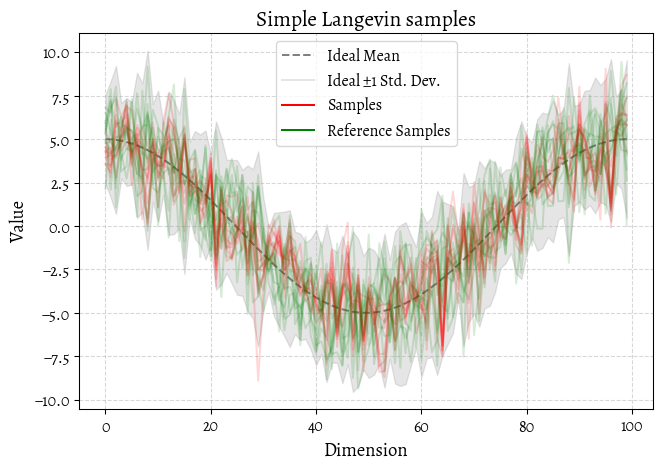

Matplotlib style set to use Alegreya font: Alegreya

That’s … mediocre. Our sampling is in the right ballpark but not playing the same game as the ideal distribution.

7 Metropolis Adjustment

When using Langevin dynamics for sampling from a probability distribution, discretization errors can lead to sampling from an incorrect distribution. We can fix this in a couple of ways. Since we know that the Gaussian target distribution is actually log-concave, we could use the implicit Langevin trick (Hodgkinson, Salomone, and Roosta 2019).

But let us try a more generic and slightly easier (but not as elegant) trick: a Metropolis-Hastings rejection step, resulting in the Metropolis-Adjusted Langevin Algorithm (MALA). This adjustment ensures that the Markov chain has the desired target distribution as its stationary distribution.

The reason we might need to do this is that when we discretized time using the Euler-Maruyama method, we introduced errors that can accumulate, causing the chain to sample from an incorrect distribution. In MALA, the proposal distribution is based on the discretized Langevin dynamics. The acceptance probability is chosen to ensure detailed balance and correct for the discretization error (thought: are these actually the same thing?).

The proposal $q(\mathbf{y}\mid \mathbf{x})$ is defined as

$$q(\mathbf{y}\mid \mathbf{x})=\mathcal{N}(\mathbf{y};\mathbf{x}-ϵ\mathrm{\nabla }U(\mathbf{x}),2ϵ\mathbf{I}).$$

The acceptance probability $\alpha (\mathbf{x},\mathbf{y})$ is given by

$$\begin{array}{rl}\alpha (\mathbf{x},\mathbf{y})& =min(1,\frac{p(\mathbf{y})q(\mathbf{x}\mid \mathbf{y})}{p(\mathbf{x})q(\mathbf{y}\mid \mathbf{x})})\\ \alpha (\mathbf{x},\mathbf{y})& =min(1,\frac{e^{-U(\mathbf{y})}\mathcal{N}(\mathbf{x};\mathbf{y}-ϵ\mathrm{\nabla }U(\mathbf{y}),2ϵ\mathbf{I})}{e^{-U(\mathbf{x})}\mathcal{N}(\mathbf{y};\mathbf{x}-ϵ\mathrm{\nabla }U(\mathbf{x}),2ϵ\mathbf{I})})\\ & =min(1,\exp (-U(\mathbf{y})+U(\mathbf{x})+\frac{1}{4ϵ}(\parallel \mathbf{y}-\mathbf{x}+ϵ\mathrm{\nabla }U(\mathbf{x}){\parallel }^2-\parallel \mathbf{x}-\mathbf{y}+ϵ\mathrm{\nabla }U(\mathbf{y}){\parallel }^2)))\end{array}$$

This ratio adjusts for the asymmetry introduced by the drift term $-ϵ\mathrm{\nabla }U(\mathbf{x})$ in the proposal distribution.

We might be worried about finding the $U(\mathbf{y})$ and $U(\mathbf{x})$ terms. Evaluating $U(\mathbf{y})=\frac{1}{2}(\mathbf{y}-\mathit{\mu }{)}^{\mathrm{\top }}{\mathrm{\Sigma }}^{-1}(\mathbf{y}-\mathit{\mu })$ directly could require forming or inverting the covariance matrix (). However, we got that term for cheap from the CG solver, since we found $\mathrm{\nabla }U(\mathbf{x})={\mathrm{\Sigma }}^{-1}(\mathbf{x}-\mathit{\mu })={\mathrm{\Sigma }}^{-1}(\mathbf{y}-\mathit{\mu })$ already; so this is simply a dot product now, $U(\mathbf{y})=\frac{1}{2}(\mathbf{y}-\mathit{\mu }{)}^{\mathrm{\top }}{\mathrm{\Sigma }}^{-1}(\mathbf{y}-\mathit{\mu })=\frac{1}{2}(\mathbf{y}-\mathit{\mu })\cdot \mathrm{\nabla }U(\mathbf{x}).$

import jax
import jax.numpy as jnp
from jax import random


def log_q(x_new, x_old, grad_old, epsilon):
    """
    Compute the log of the proposal density q(y | x).

    Parameters:
    - x_new: Proposed state (JAX array).
    - x_old: Current state (JAX array).
    - grad_old: Gradient of U at x_old (JAX array).
    - epsilon: Time step size (float).

    Returns:
    - log_q: Log of the proposal density (float).
    """
    diff = x_new - x_old + epsilon * grad_old
    return -0.25 / epsilon * jnp.dot(diff, diff)


def metropolis_adjustment(x, y, U_x, U_y, grad_x, grad_y, epsilon, key):
    """
    Perform Metropolis-Hastings acceptance step.

    Parameters:
    - x: Current state (JAX array).
    - y: Proposed state (JAX array).
    - U_x: Potential at current state (float).
    - U_y: Potential at proposed state (float).
    - grad_x: Gradient of U at x (JAX array).
    - grad_y: Gradient of U at y (JAX array).
    - epsilon: Time step size (float).
    - key: JAX PRNGKey.

    Returns:
    - x_new: Accepted or retained state (JAX array).
    """
    log_q_y_given_x = log_q(y, x, grad_x, epsilon)
    log_q_x_given_y = log_q(x, y, grad_y, epsilon)

    log_alpha = -U_y + U_x + log_q_x_given_y - log_q_y_given_x
    log_alpha = jnp.minimum(log_alpha, 0.0)  # Ensure log_alpha <= 0

    u = random.uniform(key)  # u ~ Uniform(0, 1)
    accept = u < jnp.exp(log_alpha)

    if accept:
        return y
    else:
        return x


def mala_step(x, mu, L, sig2, epsilon, key):
    """
    Perform one step of the Metropolis-Adjusted Langevin Algorithm (MALA).

    Parameters:
    - x: Current state (JAX array).
    - mu: Mean vector (JAX array).
    - L: Low-rank matrix defining Σ = L L^T + sig2 * I.
    - sig2: Variance term in Σ.
    - epsilon: Time step size (float).
    - key: JAX PRNGKey.

    Returns:
    - x_new: New state (JAX array).
    - key: Updated PRNGKey.
    """
    # Split key
    key, subkey1, subkey2 = random.split(key, num=3)

    # Compute gradient and potential at x
    r_x = x - mu
    grad_x = cg_solver(r_x, mv_prod_fn, tol=1e-5, max_iter=100)
    U_x = 0.5 * jnp.dot(r_x, grad_x)

    # Propose new state y
    noise = random.normal(subkey1, shape=x.shape)
    y = x - epsilon * grad_x + jnp.sqrt(2 * epsilon) * noise

    # Compute gradient and potential at y
    r_y = y - mu
    grad_y = cg_solver(r_y, mv_prod_fn, tol=1e-5, max_iter=100)
    U_y = 0.5 * jnp.dot(r_y, grad_y)

    # Perform Metropolis adjustment
    x_new = metropolis_adjustment(x, y, U_x, U_y, grad_x, grad_y, epsilon, subkey2)

    return x_new, key


def sample_mvn_mala(mu, L, sig2, num_samples=1000, epsilon=1e-3, burn_in=100):
    """
    Samples from N(mu, Σ) using the Metropolis-Adjusted Langevin Algorithm (MALA).

    Parameters:
    - mu: Mean vector (JAX array of shape [D]).
    - L: Low-rank matrix defining Σ = L L^T + sig2 * I.
    - sig2: Variance term in Σ.
    - num_samples: Number of samples to collect after burn-in.
    - epsilon: Time step size.
    - burn_in: Number of initial iterations to discard.

    Returns:
    - samples: Samples from the target distribution (JAX array of shape [num_samples, D]).
    """
    D = mu.shape[0]
    key = random.PRNGKey(0)

    # Random initialization
    key, subkey = random.split(key)
    # Small perturbation around mu
    x = mu + random.normal(subkey, shape=(D,)) * 0.1

    samples = []

    total_steps = burn_in + num_samples

    for n in range(total_steps):
        x, key = mala_step(x, mu, L, sig2, epsilon, key)

        # Collect samples after burn-in
        if n >= burn_in:
            samples.append(x)

    return jnp.stack(samples)

OK, now let us generate some samples using this shiny new MALA sampler.

mala_samples = sample_mvn_mala(mu, L, sig2, num_samples=500, epsilon=1e-2, burn_in=100)

ideal_std_diag = np.sqrt((L * L).sum(1) + sig2)

plot_validation(
    samples=np.array(mala_samples),
    mu=np.array(mu),
    sigma_diag=ideal_std_diag,
    reference_samples=A.T,
    title="MALA samples",
)
plt.show()

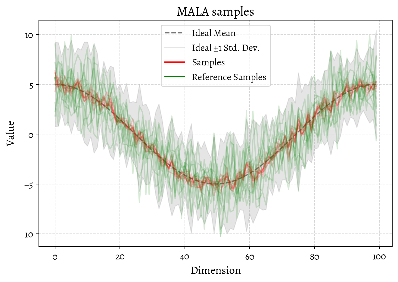
We could investigate the convergence of the MALA sampler by looking at the trace of the samples and think about trade-offs of step size and burn-in etc. I’m not inclined to do that, for a reason that I’ll expand next, which is that this is a silly way of sampling from a Gaussian distribution.

We should ask ourselves when is this method is worth trying at all. This can sample powerfully from tricky Gaussians when we can compute $\mathrm{\Sigma }\mathbf{v}$ but not $\mathrm{\Sigma }$. When can we, in fact, do that? The case here, where $\mathrm{\Sigma }=L{L}^T+{\sigma }^{2}I$ is a good example, but also kind of useless. There is a way simpler way to sample from that distribution, to wit

1. Sample $\mathbf{z}\sim \mathcal{N}(0,I)$, $\mathit{\zeta }\sim \mathcal{N}(0,I)$.
2. $\mathbf{x}=\mu +L\mathbf{z}+\sigma \mathit{\zeta }$ is a sample from $\mathcal{N}(\mu ,L{L}^T+{\sigma }^{2}I)$.

To see this, just calculate the mean and variance of $\mathbf{x}$. Very simple, very clean, no complicated solvers or burn-in or rejection steps.

So this Langevin example per se is useless (but fun, I hope). But the question might be: are there other occasions when we can calculate $\mathrm{\Sigma }\mathbf{v}$ but not $\mathrm{\Sigma }$? I cannot think of any right now; to be honest I had a vague idea that one would occur to me when I was writing this; but instead I have persuaded myself that there are no such things.

That is not to say Langevin-type dynamics are not useful; but I think we need to be cleverer; probably score diffusions, which have a very sophisticated way of sampling from punishing (and not even Gaussian) distributions are the interesting case.

8 References