Physics-informed neural networks

1 Deterministic PINN

Archetypally, the PINN. Recently these have been hip (Raissi, Perdikaris, and Karniadakis 2017a, 2017b; Raissi, Perdikaris, and Karniadakis 2019; L. Yang, Zhang, and Karniadakis 2020; Zhang, Guo, and Karniadakis 2020; Zhang et al. 2019). Zhang et al. (2019) credits Lagaris, Likas, and Fotiadis (1998) with originating the idea in 1998, so I suppose this is not super fresh. Thanks Shams Basir who has an earlier date for this. In Basir and Senocak (2022) credit goes to Dissanayake and Phan-Thien (1994) and van Milligen, Tribaldos, and Jiménez (1995). The key insight is that if we are elbows-deep in a neural network framework anyway, we already have access to automatic differentiation, so differential operations over the input field are basically free.

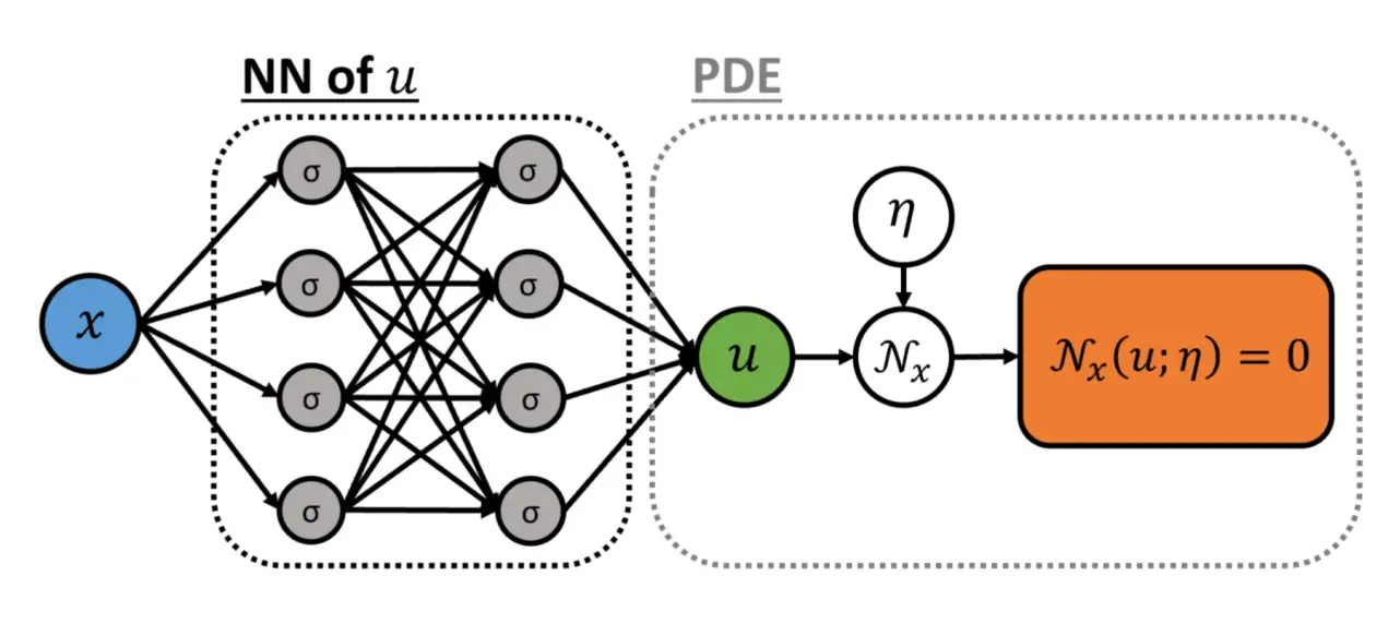
Let us introduce the basic “forward” PINN setup as given in Raissi, Perdikaris, and Karniadakis (2019): In the basic model we have the following problem $$f+\mathcal{D}[f;\eta ]=0,x\in \mathrm{\Omega },t\in [0,T]$$ where $f(t,x)$ denotes the solution (note this $\mathcal{D}$ has the opposite sign to the convention we used in the intro). We assume the differential operator $\mathcal{D}$ is parameterised by some $\eta$ which for now we take to be known and suppress. Time and space axes are not treated specially in this approach but we keep them separate so that we can more closely approximate the terminology of the original paper. Our goal is to learn a neural network $f:{\mathbb{R}}^e\to {\mathbb{R}}^d\in \mathcal{A}$ that approximates the solution to this PDE. We also assume we have some observations from the true PDE solutions, presumably simulated or analytically tractable enough to be given analytically. The latter case is presumably for benchmarking, as it makes this entire approach pointless AFAICS if the analytic version is easy.

We define residual network $r(t,x)$ to be given by the left-hand side of the above $$r:=f+\mathcal{D}[f]$$ and proceed by approximating $u(t,x;\theta )$ with a deep neural network $r(t,x;\theta )$.

The approximation is data-driven, with sample set $S_t$ from a run of the PDE solver, $$S=\{{\{f(t_f^{(i)},x_f^{(i)})\}}_{i=1}^{N_f},{\{r(t_r^{(i)},(x_r^{(i)})\}}_{i=1}^{N_r}\}.$$

$f(t,x;\theta )$ and $r(t,x;\theta )$ share parameters $\theta$ (but differ in output). This seems to be a neural implicit representation-style approach, where we learn functions on coordinates. Each parameter set for the simulator to be approximated is a new dataset, and training examples are pointwise-sampled from the solution.

The key insight is that if we are elbows-deep in a neural network framework anyway, we already have access to automatic differentiation, so differential operations over the input field are basically free.

We train by minimising a combined loss, $$L(\theta )={\mathrm{MSE}}_f(\theta )+{\mathrm{MSE}}_r(\theta )$$ where $${\mathrm{MSE}}_f=\frac{1}{N_f}\sum _{i=1}^{N_f}{|f(t_f^{(i)},x_f^{(i)})-f^{(i)}|}^2$$ and $${\mathrm{MSE}}_r=\frac{1}{N_r}\sum _{i=1}^{N_r}{\left|r(t_r^{(i)},x_r^{(i)})\right|}^2$$ Loss ${\mathrm{MSE}}_f$ corresponds to the initial and boundary data while ${\mathrm{MSE}}_r$ enforces the structure imposed by the defining differential operator at a finite set of collocation points. This trick allows us to learn an approximate solution operator which nearly enforces the desired conservation law.

An example is illustrative. Here is the reference Tensorflow interpretation from Raissi, Perdikaris, and Karniadakis (2019) for the Burger’s equation. In one space dimension, the Burger’s equation with Dirichlet boundary conditions reads $$\begin{array}{l}f+f{f}_x-(0.01/\pi )f_{xx}=0,x\in [-1,1],t\in [0,1]\\ f(0,x)=-\sin (\pi x)\\ f(t,-1)=f(t,1)=0\end{array}$$ We define $r(t,x)$ to be given by $$r:=f+f{f}_x-(0.01/\pi )f_{xx}$$

The python implementation of these two parts is essentially a naïve transcription of those equations.

def f(t, x):
    f = neural_net(tf.concat([t,x],1), weights, biases)
    return f

def r(t, x):
    f = f(t, x)
    f_t = tf.gradients(f, t)[0]
    f_x = tf.gradients(f, x)[0]
    f_xx = tf.gradients(f_x, x)[0]
    r = f_t + f∗f_x − (0.01/ tf.pi)∗f_xx
    return r

Because the outputs are parameterised by coordinates, the built-in autodiff does all the work. The authors summarize the resulting network topology so:

What has this gained us? So far, we have acquired a model which can, the authors assert, solve deterministic PDEs, which is nothing we could not do before. We have sacrificed any guarantee that our method will in fact do well on data from outside our observations. Also, I do not understand how I can plug alternative initial or boundary conditions into this. There is no data input, as such, at inference time, merely coordinates. On the other hand, the authors assert that this is faster and more stable than traditional solvers. It has the nice feature that the solution is continuous in its arguments; there is no grid. As far as NN things go, the behaviour of this model is weird and refreshing: it is simple, requires small data, and has few tuning parameters.

But! what if we don’t know the parameters of the PDE? Assume the differential operator has parameter $\eta$ which is not in fact known. $$f+\mathcal{D}[f;\eta ]=0,x\in \mathrm{\Omega },t\in [0,T]$$ The trick, as far as I can tell, is simply to include $\eta$ in trainable parameters. $$r(\eta ):=f(\eta )+\mathcal{D}[f;\eta ]$$ and proceed by approximating $f(t,x;\theta ,\eta )$ with a deep neural network $r(t,x;\theta ,\eta )$. Everything else proceeds as before.

Fine; now what? Two obvious challenges from where I am sitting.

1. No way of changing inputs in the sense of initial or boundary conditions, without re-training the model
2. Point predictions. No accounting for randomness or uncertainty.

2 Stochastic PINN

Zhang et al. (2019) address point 2 via chaos expansions to handle the PDE emulation as a stochastic process regression, which apparently gives us estimates of parametric and process uncertainty. All diagrams in this section come from that paper.

🏗️ Terminology warning: I have not yet harmonised the terminology of this section with the rest of the page.

The extended model adds a random noise parameter $k(x;\omega )$: $$\begin{array}{c}{\mathcal{D}}_x[u(x;\omega );k(x;\omega )]=0,x\in \mathcal{D},\omega \in \mathrm{\Omega }\\ \text{ B.C. }{\mathcal{B}}_x[u(x;\omega )]=0,x\in \mathrm{\Gamma }\end{array}$$

The randomness in this could indicate a random coupling term, or uncertainty in some parameter of the model. Think of a Gaussian process prior over the forcing term of the PDE. We sample this noise parameter also and augment the data set with it, over $N$ distinct realisations, giving a data set like this:

$$S={\{{\{k(t_u^{(i)},x_u^{(i)};{\omega }_s)\}}_{i=1}^{N_u},{\{u(t_u^{(i)},x_u^{(i)};{\omega }_s)\}}_{i=1}^{N_u},{\{r(t_r^{(i)},(x_r^{(i)})\}}_{i=1}^{N_r}\}}_{s=1}^N.$$

Note that I have kept the time variable explicit, unlike the paper, to match the previous section, but it gets cluttered if we continue to do this, so let’s suppress $t$ hereafter, and make it just another axis of a multidimensional $x$.

So now we approximate $k$. Why? AFAICT that is because we are going to make a polynomial basis for $\xi$ which means that we want few dimensions.

We let $K$ be the $N_k\times N_k$ covariance matrix for the sensor measurements on $k,$ i.e., $$K_{i,j}=\mathrm{Cov}(k^{(i)},k^{(j)})$$ We take an eigendecomposition of $K$. Let ${\lambda }_l$ and ${\varphi }_l$ denote $l$-th largest eigenvalue and its associated normalized eigenvector of Then we have $$K={\mathrm{\Phi }}^T\mathrm{\Lambda }\mathrm{\Phi }$$ where $\mathbf{\Phi }=[{\varphi }_1,{\varphi }_2,\dots ,{\varphi }_{N_k}]$ is an orthonormal matrix and $\mathbf{\Lambda }=\mathrm{diag}({\lambda }_1,{\lambda }_2,\dots {\lambda }_{N_k})$ is a diagonal matrix. Let ${\mathit{k}}_s={[k_s^{(1)},k_s^{(2)},\dots ,k_s^{\left(N_k\right)}]}^T$ be the results of the $k$ measurements of the $s$-th snapshot, then $${\mathit{\xi }}_s={\mathbf{\Phi }}^T{\sqrt{\mathbf{\Lambda }}}^{-1}{\mathit{k}}_s$$ is a whitened, i.e. uncorrelated, random vector, and hence ${\mathit{k}}_s$ can be rewritten as a reduced dimensional expansion $${\mathit{k}}_s\approx {\mathit{k}}_0+\sqrt{{\mathbf{\Lambda }}^M}{\mathbf{\Phi }}^M{\mathit{\xi }}_s^M,M<N_k$$ where ${\mathit{k}}_0=\mathbb{E}\mathit{k}.$ We fix $M\ll N_k$ and suppress it hereafter.

Now we have approximated away the correlated $\omega$ noise and in favour of this $\xi$ which we have finite-dimensional representations of. $$k(x_k^{(i)};{\omega }_s)\approx k_0\left(x_k^{(i)}\right)+\sum _{l=1}^M\sqrt{{\lambda }_l}{k}_l\left(x_k^{(i)}\right){\xi }_{s,l},M<N_k$$ Note that this is defined only at the observation points, though.

Next is where we use the chaos expansion trick to construct an interpolant. Suppose the measure of RV $\xi$ is $\rho$. We approximate this unknown measure by its empirical measure $ {S}$.$$ () {S}()= {{s} S} {{s}}() $$ where ${\delta }_{{\xi }_s}$ is the Dirac measure.

We construct a polynomial basis which is orthogonal with respect to the inner product associated to this measure, specifically $$\begin{array}{rl}⟨\varphi ,\psi ⟩& :=\int \varphi (x)\psi (x)\rho (x)\mathrm{d}x\\ & \approx \int \varphi (x)\psi (x){\nu }_S(x)\mathrm{d}x\end{array}$$

OK, so we construct an orthonormal polynomial basis ${\{{\psi }_{\alpha }(\mathit{\xi })\}}_{\alpha =0}^P$ via the Gram-Schmidt orthogonalization process.¹ With the polynomial basis $\{{\psi }_{\alpha }(\mathit{\xi })\}$ we can write a function $g(x;\mathit{\xi })$ in the form of the aPC expansion, $$g(x;\mathit{\xi })=\sum _{\alpha =0}^P{g}_{\alpha }(x){\psi }_{\alpha }(\mathit{\xi })$$ where each $g_{\alpha }(x)$ is calculated by $$g_{\alpha }(x)=\frac{1}{N}\sum _{s=1}^N{\psi }_{\alpha }\left({\mathit{\xi }}_s\right)g(x;{\mathit{\xi }}_s).$$

So we are going to pick $g$ to be some quantity of interest in our sim, and in fact, we take it to be two separate quantities, $u$ and $k$.

Then, we can approximate $k$ and $u$ at the $s$-th snapshot by $$\tilde{k}(x;{\omega }_s)=\widehat{k_0}(x)+\sum _{i=1}^M\sqrt{{\lambda }_i}\widehat{k_i}(x){\xi }_{s,i}$$ and $$\tilde{u}(x;{\omega }_s)=\sum _{\alpha =0}^P\widehat{u_{\alpha }}(x){\psi }_{\alpha }\left({\mathit{\xi }}_s\right).$$

We construct two networks,

1. the network $\widehat{u_{\alpha }}$, which takes the coordinate $x$ as the input and outputs a $(P+1)\times 1$ vector of the aPC modes of $u$ evaluated at $x$, and
2. the network $\widehat{k_i}$ that takes the coordinate $x$ as the input and outputs a $(M+1)\times 1$ vector of the $k$ modes.

The resulting network topology is

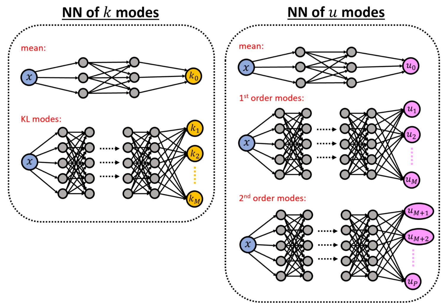
For concreteness, here is the topology for an example problem $\mathcal{D}:=-\frac{\mathrm{d}}{\mathrm{d}x}(k(x;\omega )\frac{\mathrm{d}}{\mathrm{d}x}u)-f$:

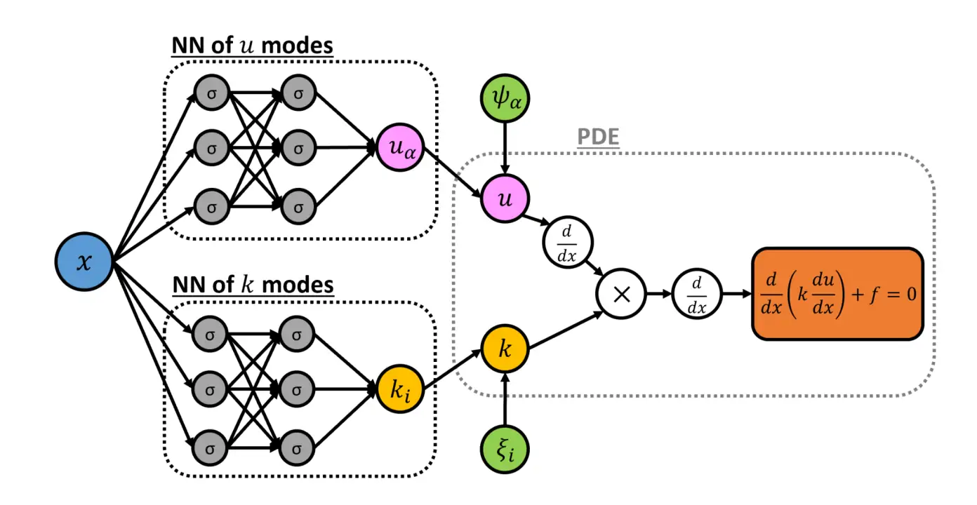
At inference time we take observations of $k$, calculate the whitened $\xi$, then use the chaos expansion representation to calculate the values at unobserved locations. $$\mathcal{L}\left(S_t\right)={\mathrm{MSE}}_u+{\mathrm{MSE}}_k+{\mathrm{MSE}}_f$$ where $$\begin{array}{l}{\mathrm{MSE}}_u=\frac{1}{N{N}_u}\sum _{s=1}^N\sum _{i=1}^{N_u}\left[{(\tilde{u}(x_u^{(i)};{\omega }_s)-u(x_u^{(i)};{\omega }_s))}^2\right]\\ {\mathrm{MSE}}_k=\frac{1}{N{N}_k}\sum _{s=1}^N\sum _{i=1}^{N_k}\left[{(\tilde{k}(x_k^{(i)};{\omega }_s)-k(x_k^{(i)};{\omega }_s))}^2\right]\end{array}$$ and $${\mathrm{MSE}}_f=\frac{1}{N{N}_f}\sum _{s=1}^N\sum _{i=1}^{N_f}\left[{\left({\mathcal{D}}_x[\tilde{u}(x_f^{(i)};{\omega }_s);\tilde{k}(x_f^{(i)};{\omega }_s)]\right)}^2\right]$$

After all that I would describe this as a method to construct a stochastic PDE with the desired covariance structure, which is a hard thing to do. OK, all that was very complicated. Although, it was a complicated thing to do; Consider the mess this gets us into in the Karhunen Loéve expansion and spectral expansion Anyway, after all this, presuming the neural networks are perfect, we have a good estimate of the distribution of random parameters and random output of a stochastic PDE evaluated over the whole surface from partial discrete measurements.

How do we estimate the uncertainty introduced by the neural net? Dropout.

Further questions:

1. Loss scale; gradient errors may not be comparable to value errors in the loss function.
2. Network capacity: What size networks are necessary (not the ones we learn are tiny, with only hundreds of parameters)
3. How do we generalize this to different initial conditions? Can we learn an observation-conditional PDE?
4. After all this work it looks like I still can’t do inference on this thing. How do I update a distribution over $k$ by this method from observations of a new PDE?
5. Notice how the parameter inference problem for $\eta$ vanished for the stochastic PDE? Can we learn an estimate for $u$, $\eta$ and $k$ simultaneously in this setting? I imagine we repeat the trick where that parameter is learned along with the $u$ network.

3 Weak formulation

TODO: should this be filed with PINNs?

A different network topology using the implicit representation trick is explored in Zang et al. (2020) and extended to inverse problems in Bao et al. (2020), They discuss this in terms of a weak formulation of a PDE.

🏗️ Terminology warning: I have not yet harmonised the terminology of this section with the rest of the page.

We start with the example second-order elliptic² PDE with on domain $\mathrm{\Omega }\subset {\mathbb{R}}^d$ given $$\mathcal{D}[u]-f:=-\sum _{i=1}^d{\partial }_i\left(\sum _{j=1}^d{a}_{ij}{\partial }_{j}u\right)+\sum _{i=1}^d{b}_i{\partial }_{i}u+cu-f=0$$ where $a_{ij},b_i,c:\mathrm{\Omega }\to \mathbb{R}$ for $i,j\in [d]\triangleq \{1,\dots ,d\},f:\mathrm{\Omega }\to \mathbb{R}$ and $g:\partial \mathrm{\Omega }\to \mathbb{R}$ are all given. We start by assuming Dirichlet boundary conditions, $u(x)-g(x)=0$, although this is rapidly generalised.

By multiplying both sides by a test function $\phi \in H_0^1(\mathrm{\Omega };\mathbb{R})$ and integrating by parts: $$\{\begin{array}{l}⟨\mathcal{D}[u],\phi ⟩\triangleq {\int }_{\mathrm{\Omega }}(\sum _{j=1}^d\sum _{i=1}^d{a}_{ij}{\partial }_{j}u{\partial }_i\phi +\sum _{i=1}^d{b}_i\phi {\partial }_{i}u+cu\phi -f\phi )\mathrm{d}x=0\\ \mathcal{B}[u]=0,\text{ on }\partial \mathrm{\Omega }\end{array}$$

The clever insight is that this inspires an adversarial problem to find the weak solutions, by considering the $L^2$ operator norm of $\mathcal{D}[u](\phi )\triangleq ⟨\mathcal{D}[u],\phi ⟩$. Then the operator norm of $\mathcal{D}[u]$ is defined $$\parallel \mathcal{D}[u]{\parallel }_{op}\triangleq max\{⟨\mathcal{D}[u],\phi ⟩/\parallel \phi {\parallel }_2\mid \phi \in H_0^1,\phi \ne 0\}.$$ Therefore, $u$ is a weak solution of the PDE if and only if $\parallel \mathcal{D}[u]{\parallel }_{op}=0$ and the boundary condition $\mathcal{B}[u]=0$ is satisfied on $\delta \mathrm{\Omega }$. As $\parallel \mathcal{D}[u]{\parallel }_{op}\ge 0$, we know that a weak solution $u$ thus solves the following two equivalent problems in observation: $$\underset{u\in H^1}{min}\parallel \mathcal{D}[u]{\parallel }_{op}^2⟺\underset{u\in H^1}{min}\underset{\phi \in H_0^1}{max}|⟨\mathcal{D}[u],\phi ⟩{|}^2/\parallel \phi {\parallel }_2^2.$$

Specifically the solutions $u_{\theta }:{\mathbb{R}}^d\to \mathbb{R}$ are realized as a deep neural network with parameter $\theta$ to be learned, such that $\mathcal{S}\left[u_{\theta }\right]$ minimizes the (estimated) operator norm. The test function $\phi$, is a deep adversarial network with parameter $, which adversarially challenges $u_{\theta }$ by maximising $⟨\mathcal{D}\left[u_{\theta }\right],{\phi }_{\eta }⟩/{\Vert {\phi }_{\eta }\Vert }_2$ for every given $u_{\theta }$.

To train the deep neural network $u_{\theta }$ and the adversarial network ${\phi }_{\eta }$ we construct appropriate loss functions $u_{\theta }$ and ${\phi }_{\eta }$. Since the logarithm function is monotone and strictly increasing, we can for convenience formulate the objective of $u_{\theta }$ and ${\phi }_{\eta }$ in the interior of $\mathrm{\Omega }$ as $$L_{\text{int }}(\theta ,\eta )\triangleq \log {\left|⟨\mathcal{D}\left[u_{\theta }\right],{\phi }_{\eta }⟩\right|}^2-\log {\Vert {\phi }_{\eta }\Vert }_2^2.$$ In addition, the weak solution $u_{\theta }$ must also satisfy the boundary condition $\mathcal{B}[u]=0$ on $\delta \mathrm{\Omega }$ which we fill in as above, calling it $L_{\text{bdry }}(\theta ).$ The total adversarial objective function is the weighted sum of the two objectives for which we seek for a saddle point that solves the minimax problem: $$\underset{o}{min}maxL(\theta ,\eta ),\text{ where }L(\theta ,\eta )\triangleq L_{\text{int }}(\theta ,\eta )+\alpha L_{\text{bdry }}(\theta ).$$ $\alpha$ might seem arbitrary; apparently it is useful as a tuning parameter.

This is a very elegant idea, although the implicit representation thing is still a problem for my use cases.

4 PINO

Combines operator learning with physics-informed neural networks. Li et al. (2021):

Code at neuraloperator/PINO.

5 Implementation

• pytorch via TorchPhysics

• Tensorflow

  • DeepXDE
  • source

6 Incoming

• idrl-lab/PINNpapers: Must-read Papers on Physics-Informed Neural Networks.
• X. Chen et al. (2021) uses an attention mechanism to improve the performance of PINNs. I’m curious.
• Introduction to Scientific Machine Learning 2: Physics-Informed Neural Networks
• Introduction to Scientific Machine Learning through Physics-Informed Neural Networks

7 References