Transforms of Gaussian noise

1 Taylor expansion

Not complicated but it can be a little subtle. For a general exposition which handles first and second-order transforms, I recommend Gustafsson and Hendeby (2012), which as a bonus proves some things which seem obvious but are not, in fact, obvious to prove, and disproves some things which seemd obviously true to me. Arras (1998) is possibly the most simple introduction.

Taylor expansion works if the transformation in question is smooth enough and the approximation only needs to be accurate about the expansion point.

Todo: treat expansion point and mean separately.

Consider a general nonlinear differentiable transformation \(g\) and its second order Taylor expansion. We apply \(g:\mathbb{R}^{n_{x}}\to\mathbb{R}^{n_{z}}\) to a variable \(x,\) defining \(z:=g(x).\) Let \(\mathrm{E}(x)=\mu_{x}\) and \(\operatorname{Var}(x)=P_{x}.\) The Hessian of the \(i^{\text {th }}\) component of \(g\) is denoted \(g_{i}^{\prime \prime}.\) \([x_i]_i\) is a vector where the \(i\)th element is \(x_i\). We approximate \(z\) using the Taylor expansion, \[z=g\left(\mu_{x}\right)+g^{\prime}\left(\mu_{x}\right)\left(x-\mu_{x}\right)+\left[\frac{1}{2}\left(x-\mu_{x}\right)^{T} g_{i}^{\prime \prime}\left(\mu_{x}\right)\left(x-\mu_{x}\right)\right]_{i}.\] Leaving aside questions of when this is convergent for now, and assume it is. Then we assert \(z\sim\mathcal{N}(\mu_z,P_z)\). The first moment of \(z\) is given by \[ \mu_{z}=g\left(\mu_{x}\right)+\frac{1}{2}\left[\operatorname{tr}\left(g_{i}^{\prime \prime}\left(\mu_{x}\right) P_{x}\right)\right]_{i} \] Further, let \(x \sim \mathcal{N}\left(\mu_{x}, P_{x}\right)\), then the second moment of \(z\) is given by \[ P_{z}=g^{\prime}\left(\mu_{x}\right) P_{x}\left(g^{\prime}\left(\mu_{x}\right)\right)^{T}+\frac{1}{2}\left[\operatorname{tr}\left(g_{i}^{\prime \prime}\left(\mu_{x}\right) P_{x} g_{j}^{\prime \prime}\left(\mu_{x}\right) P_{x}\right)\right]_{i j} \] with \(i, j=1, \ldots, n_{z}.\)

This approach is finite dimensional, but it also generalises to Gaussian processes, in that we can, at any finite number of test locations, once again find a first order approximation. See the non-parametric case.

Note that here I have assumed that we have the luxury of expanding the distribution about the mean, which would be a factor encouraging me to attempt to get away with only taking the first order Taylor transform. Since I have bothered to take a second-order expansion here, I should give the expansion about an arbitrary point which is not necessarily the mean, for the sake of making the generality worth it.

Question: In what metric, if any, have we minimised the error of our approximation by doing this?

• Robert Grosse’s lectures on CSC2541 Topics in Machine Learning: Neural Net Training Dynamics includes IMO the best introduction to applied Taylor expansions in arbitrary dimension here.
• Byron Boots’ lecture on the extended Kalman filter.

2 Monte Carlo moment matching

Classic Monte Carlo methods use a sample to approximate the moments of a distribution, as seen in ensemble Kalman methods.

3 Monte Carlo gradient descent in some metric

If we choose some Monte Carlo method then we can use gradient information to approximate the target in any useful probability metric). This is not special to Gaussian processes, but works with any old stochastic variational method.

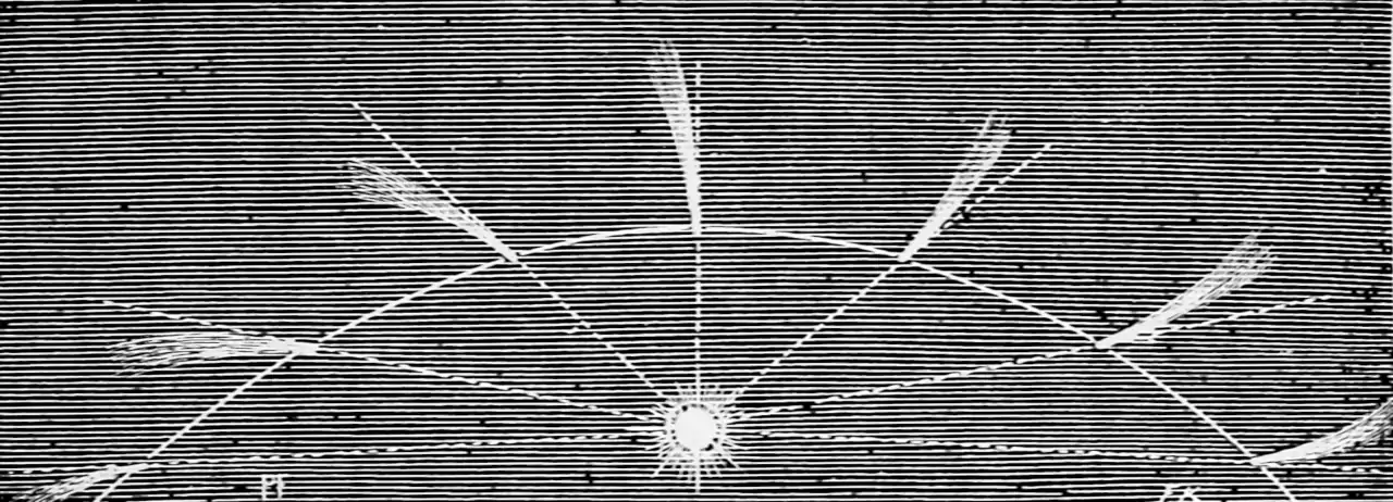
4 Unscented transform

The great invention of Uhlmann and Julier is the unscented transform, which uses a cunningly-chosen non-random empirical sample at so-called sigma-points to approximate the transformed distribution via its moments. I think that anything using sigma points is an unscented transform? Otherwise it is just garden-variety moment-matching.

Often seen in the context of Kalman filtering.

What the Unscented Transform does is to replace the mean vector and its associated error covariance matrix with a special set of points with the same mean and covariance. In the case of the mean and covariance representing the current position estimate for a target, the UT is applied to obtain a set of points, referred to as sigma points, to which the full nonlinear equations of motion can be applied directly. In other words, instead of having to derive a linearized approximation, the equations could simply be applied to each of the points as if it were the true state of the target. The result is a transformed set of points, and the mean and covariance of that set represents the estimate of the predicted state of the target.

See, e.g., Roth, Hendeby, and Gustafsson (2016) and a comparison with the Taylor expansion in Gustafsson and Hendeby (2012).

Question: What would we need to do to apply the unscented transform to non-Gaussian distributions? See Ebeigbe et al. (2021).

• Unscented transform
• The Unscented Transform
• Unscented Kalman Filter

5 Subsampled

See GP by GD.

6 Fisher information

Fisher information between two Gaussians

7 Chaos expansions

See chaos expansions.

8 Gaussian processes

Propagating error of Gaussian process inputs is a functional GP problem. TBD.

Related, propagating error through a GP regression. See Emmanuel Johnson’s Linearized GP site (mildly idiosyncratic notation and very idiosyncratic website navigation).

The following references from Emmanuel Johnson’s lit review look promising: Deisenroth and Mohamed (2012);Girard and Murray-Smith (2003);Ko and Fox (2009) and McHutchon and Rasmussen (2011).

I am curious what, if anything, they add to Murray-Smith and Pearlmutter (2005).

9 References