Approximate matrix factorisations and decompositions
Sometimes even exact
2014-08-05 — 2023-08-23
Wherein Approximate Matrix Factorisations Are Surveyed and Low-Rank-Plus-Sparse Decompositions, Randomised Sketching and Lanczos Approximations Are Presented as Practical Routes to Scalable Matrix Approximation.
Assumed audience:
People with undergrad linear algebra
1 The classics
The big six exact matrix decompositions are (Stewart 2000)
- Cholesky decomposition
- pivoted LU decomposition
- QR decomposition
- spectral decomposition
- Schur decomposition; and
- singular value decomposition.
See Nick Higham’s summary of those.
2 Approximate decompositions
Mastered QR and LU decompositions? There are now so many ways of factorising matrices that there are not enough acronyms in the alphabet to hold them, especially if we suspect our matrix is sparse, or could be made sparse because of some underlying constraint, or probably could, if squinted at in the right fashion, be such as a graph transition matrix, or Laplacian, or noisy transform of some smooth object, or at least would be close to sparse if we chose the right metric, or…
A big matrix is close to, in some sense, the (tensor/matrix) product (or sum, or…) of some matrices that are in some way simple (small-rank, small dimension, sparse), possibly with additional constraints. Can we find those simple matrices?
Ethan Epperly’s introduction to Low-rank Matrices puts many ideas clearly.
Here’s an example: Godec (T. Zhou and Tao 2011) — A decomposition into low-rank and sparse components which loosely speaking, combines multidimensional factorisation and outlier detection.
GoDec is one of the most efficient algorithms for low-rank and sparse decomposition thanks to bilateral random projections (BRP), a fast approximation of SVD/PCA.
There are so many more of these things, depending on our preferred choice of metric, constraints, free variables and such.
Keywords: Matrix sketching, low-rank approximation, traditional dimensionality reduction.
Matrix concentration inequalities turn out to be a useful tool to prove that a given matrix decomp is not too bad in a PAC-sense.
Igor Carron’s Matrix Factorization Jungle classifies the following problems as matrix-factorisation type.
- Kernel Factorizations
- …
- Spectral clustering
- \([\mathrm{A} = \mathrm{D} \mathrm{X}]\) with unknown \(\mathrm{D}\) and \(\mathrm{X}\), solve for sparse \(\mathrm{X}\) and \(\mathrm{X}_i = 0\) or \(1\)
- K-Means / K-Median clustering
- \([\mathrm{A} = \mathrm{D} \mathrm{X}]\) with unknown \(\mathrm{D}\) and \(\mathrm{X}\), solve for \(\mathrm{X} \mathrm{X}^{\top} = \mathrm{I}\) and \(\mathrm{X}_i = 0 or 1\)
- Subspace clustering
- \([\mathrm{A} = \mathrm{A} \mathrm{X}]\) with unknown \(\mathrm{X}\), solve for sparse/other conditions on \(\mathrm{X}\)
- Graph Matching
- \([\mathrm{A} = \mathrm{X} \mathrm{B} \mathrm{X} ^{\top}]\) with unknown \(\mathrm{X}\), \(\mathrm{B}\) solve for \(\mathrm{B}\) and \(\mathrm{X}\) as a permutation
- NMF
- \([\mathrm{A} = \mathrm{D} \mathrm{X}]\) with unknown \(\mathrm{D}\) and \(\mathrm{X}\), solve for elements of \(\mathrm{D}\),\(\mathrm{X}\) positive
- Generalized Matrix Factorization
- \([\mathrm{W}.*\mathrm{L} − \mathrm{W}.*\mathrm{U} \mathrm{V}']\) with \(\mathrm{W}\) a known mask, \(\mathrm{U}\),\(\mathrm{V}\) unknowns solve for \(\mathrm{U}\),\(\mathrm{V}\) and \(\mathrm{L}\) lowest rank possible
- Matrix Completion
- \([\mathrm{A} = \mathrm{H}.*\mathrm{L}]\) with \(\mathrm{H}\) a known mask, \(\mathrm{L}\) unknown solve for \(\mathrm{L}\) lowest rank possible
- Stable Principle Component Pursuit (SPCP)/ Noisy Robust PCA
- \([\mathrm{A} = \mathrm{L} + \mathrm{S} + \mathrm{N}]\) with \(\mathrm{L}\), \(\mathrm{S}\), \(\mathrm{N}\) unknown, solve for \(\mathrm{L}\) low rank, \(\mathrm{S}\) sparse, \(\mathrm{N}\) noise
- Robust PCA
- \([\mathrm{A} = \mathrm{L} + \mathrm{S}]\) with , unknown, solve for \(\mathrm{L}\) low rank, \(\mathrm{S}\) sparse
- Sparse PCA
- \([\mathrm{A} = \mathrm{D} \mathrm{X} ]\) with unknown \(\mathrm{D}\) and \(\mathrm{X}\), solve for sparse \(\mathrm{D}\)
- Dictionary Learning
- \([\mathrm{A} = \mathrm{D} \mathrm{X}]\) with unknown \(\mathrm{D}\) and \(\mathrm{X}\), solve for sparse \(\mathrm{X}\)
- Archetypal Analysis
- \([\mathrm{A} = \mathrm{D} \mathrm{X}]\) with unknown \(\mathrm{D}\) and \(\mathrm{X}\), solve for \(\mathrm{D}= \mathrm{A} \mathrm{B}\) with \(\mathrm{D}\), \(\mathrm{B}\) positive
- Matrix Compressive Sensing (MCS)
- find a rank-r matrix \(\mathrm{L}\) such that \([\mathrm{A}(\mathrm{L}) ~= b]\) / or \([\mathrm{A}(\mathrm{L}+\mathrm{S}) = b]\)
- Multiple Measurement Vector (MMV)
- \([\mathrm{Y} = \mathrm{A} \mathrm{X}]\) with unknown \(\mathrm{X}\) and rows of \(\mathrm{X}\) are sparse
- Compressed sensing
- \([\mathrm{Y} = \mathrm{A} \mathrm{X}]\) with unknown \(\mathrm{X}\) and rows of \(\mathrm{X}\) are sparse, \(\mathrm{X}\) is one column.
- Blind Source Separation (BSS)
- \([\mathrm{Y} = \mathrm{A} \mathrm{X}]\) with unknown \(\mathrm{A}\) and \(\mathrm{X}\) and statistical independence between columns of \(\mathrm{X}\) or subspaces of columns of \(\mathrm{X}\)
- Partial and Online SVD/PCA
- …
- Tensor Decomposition
- Many, many options; see tensor decompositions for some tractable ones.
Truncated Classic PCA is clearly also an example, but is excluded from the list for some reason. Boringness? the fact it’s a special case of Sparse PCA?
I also add
- Square root
- \(\mathrm{Y} = \mathrm{X}^{\top}\mathrm{X}\) for \(\mathrm{Y}\in\mathbb{R}^{N\times N}, X\in\mathbb{R}^{N\times n}\), with (typically) \(n<N\).
That is a whole thing; see matrix square root.
See also learning on manifolds, compressed sensing, optimisation random linear algebra and clustering, penalised regression…
3 Tutorials
- Data mining seminar: Matrix sketching
- Kumar and Schneider have a literature survey on low rank approximation of matrices (Kumar and Shneider 2016)
- Preconditioning tutorial by Erica Klarreich
- Andrew McGregor’s ICML Tutorial Streaming, sampling, sketching
- more at signals and graph.
- Another one that makes the link to clustering is Chris Ding’s Principal Component Analysis and Matrix Factorizations for Learning
- Igor Carron’s Advanced Matrix Factorization Jungle.
4 Non-negative matrix factorisations
5 Why is approximate factorisation ever useful?
For certain types of data matrix, here is a suggestive observation: Udell and Townsend (2019) ask “Why Are Big Data Matrices Approximately Low Rank?”
Matrices of (approximate) low rank are pervasive in data science, appearing in movie preferences, text documents, survey data, medical records, and genomics. While there is a vast literature on how to exploit low rank structure in these datasets, there is less attention paid to explaining why the low rank structure appears in the first place. Here, we explain the effectiveness of low rank models in data science by considering a simple generative model for these matrices: we suppose that each row or column is associated to a (possibly high dimensional) bounded latent variable, and entries of the matrix are generated by applying a piecewise analytic function to these latent variables. These matrices are in general full rank. However, we show that we can approximate every entry of an \(m\times n\) matrix drawn from this model to within a fixed absolute error by a low rank matrix whose rank grows as \(\mathcal{O}(\log(m+n))\). Hence any sufficiently large matrix from such a latent variable model can be approximated, up to a small entrywise error, by a low rank matrix.
Ethan Epperly argues from a function approximation perspective (e.g.) that we can deduce this property from smoothness of functions.
Saul (2023) connects non-negative matrix factorisation to geometric algebra and linear algebra via deep learning and kernels. That sounds like fun.
6 As regression
Total Least Squares (a.k.a. orthogonal distance regression, or error-in-variables least-squares linear regression) is a low-rank matrix approximation that minimises the Frobenius divergence from the data matrix. Who knew?
Various other dimensionality reduction techniques can be put in a regression framing, notable Exponential-family PCA.
7 Sketching
“Sketching” is a common term to describe a certain type of low-rank factorisation, although I am not sure which types. 🏗
(Martinsson 2016) mentions CUR and interpolative decompositions. What is that now?
8 Randomization
Rather than find an optimal solution, why not just choose a random one which might be good enough? There are indeed randomised versions, and many algorithms are implemented using randomness and in particular low-dimensional projections.
9 Connections to kernel learning
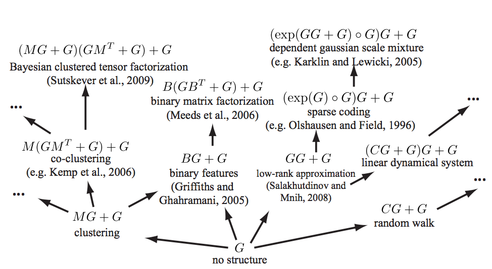
See (Grosse et al. 2012) for a mind-melting compositional matrix factorization diagram, constructing a search over hierarchical kernel decompositions that also turn out to have some matrix factorisation interpretations.
10 Bayesian
Nakajima and Sugiyama (2012):
Mnih and Salakhutdinov (2008) proposed a Bayesian maximum a posteriori (MAP) method based on the Gaussian noise model and Gaussian priors on the decomposed matrices. This method actually corresponds to minimising the squared-loss with the trace-norm penalty (Srebro, Rennie, and Jaakkola 2004) Recently, the variational Bayesian (VB) approach (Attias 1999) has been applied to MF (Lim and Teh 2007; Raiko, Ilin, and Karhunen 2007), which we refer to as VBMF. The VBMF method was shown to perform very well in experiments. However, its good performance was not completely understood beyond its experimental success.
☜ Insert further developments here. Possibly Brouwer’s thesis (Brouwer 2017) or Shakir Mohamed’s (Mohamed 2011) would be a good start, or Benjamin Drave’s tutorial, Probabilistic Matrix Factorization and Xinghao Ding, Lihan He, and Carin (2011).
I am currently sitting in a seminar by He Zhao on Bayesian matrix factorisation, wherein he is building up this tool for discrete data, which is an interesting case. He starts from M. Zhou et al. (2012) and builds up to Zhao et al. (2018), introducing some hierarchical descriptions along the way. His methods seem to be sampling-based rather than variational (?).
Generalized² Linear² models (Gordon 2002) unify nonlinear matrix factorisations with Generalized Linear Models. I had not heard of that until recently; I wonder how common it is?
11 Lanczos decomposition
Lanczos decomposition is a handy approximation for matrices which are cheap to multiply because of some structure, but expensive to store. It can also be used to calculate an approximate inverse cheaply.
See Krylov subspace methods for more on this.
12 Estimating rank
Eigencount and Numerical Rank
If \(f: \lambda \mapsto \mathbf{1}_{[a, b]}(\lambda)\) is the indicator (step) function in the interval \([a, b]\), then \(\operatorname{trace}(\mathbf{1}(\mathbf{A}))\) estimates the number of non-zero eigenvalues of \(\mathbf{A}\) in that interval, which is an inexpensive method to estimate the rank of a large matrix. Eigencount is closely related to the Principal Component Analysis (PCA) and low-rank approximations in machine learning.
13 Incremental decompositions
13.1 SVD
See incremental SVD.
13.2 Cholesky
14 Low rank plus diagonal
Specifically \((\mathrm{K}=\mathrm{Z} \mathrm{Z}^{\top}+\sigma^2\mathrm{I})\) where \(\mathrm{K}\in\mathbb{R}^{N\times N}\) and \(\mathrm{Z}\in\mathbb{R}^{N\times D}\) with \(D\ll N\). A workhorse.
Lots of fun tricks.
15 Misc
- Nick Higham, What Is a Rank-Revealing Factorization?
16 As an optimisation problem
There are some generalised optimisation problems which look useful for matrix factorisation, e.g. Bhardwaj, Klep, and Magron (2021):
Polynomial optimization problems (POP) are prevalent in many areas of modern science and engineering. The goal of POP is to minimize a given polynomial over a set defined by finitely many polynomial inequalities, a semialgebraic set. This problem is well known to be NP-hard, and has motivated research for more practical methods to obtain approximate solutions with high accuracy.[…]
One can naturally extend the ideas of positivity and sums of squares to the noncommutative (nc) setting by replacing the commutative variables \(z_1, \dots , z_n\) with noncommuting letters \(x_1, \dots , x_n\). The extension to the noncommutative setting is an inevitable consequence of the many areas of science which regularly optimize functions with noncommuting variables, such as matrices or operators. For instance in control theory, matrix completion, quantum information theory, or quantum chemistry
Matrix calculus can help sometimes.
17 \([\mathcal{H}]\)-matrix methods
It seems like low-rank matrix factorisation could be related to \([\mathcal{H}]\)-matrix methods, but I do not know enough to say more.
See hmatrix.org for one lab’s backgrounder and their implementation, h2lib, hlibpro for a black-box closed-source one.
18 Tools
In pytorch, various operations are made easier with cornellius-gp/linear_operator.
Ameli’s tools:
NMF Toolbox (MATLAB and Python):
Nonnegative matrix factorization (NMF) is a family of methods widely used for information retrieval across domains including text, images, and audio. Within music processing, NMF has been used for tasks such as transcription, source separation, and structure analysis. Prior work has shown that initialization and constrained update rules can drastically improve the chances of NMF converging to a musically meaningful solution. Along these lines we present the NMF toolbox, containing MATLAB and Python implementations of conceptually distinct NMF variants—in particular, this paper gives an overview for two algorithms. The first variant, called nonnegative matrix factor deconvolution (NMFD), extends the original NMF algorithm to the convolutive case, enforcing the temporal order of spectral templates. The second variant, called diagonal NMF, supports the development of sparse diagonal structures in the activation matrix. Our toolbox contains several demo applications and code examples to illustrate its potential and functionality. By providing MATLAB and Python code on a documentation website under a GNU-GPL license, as well as including illustrative examples, our aim is to foster research and education in the field of music processing.
Vowpal Wabbit factors matrices, e.g. for recommender systems. It seems the --qr version is more favoured.
HPC for matlab, R, python, c++: libpmf:
LIBPMF implements the CCD++ algorithm, which aims to solve large-scale matrix factorization problems such as the low-rank factorization problems for recommender systems.
Spams (C++/MATLAB/python) includes some matrix factorisations in its sparse approx toolbox. (see optimisation)
scikit-learn (python) does a few matrix factorisation in its inimitable batteries-in-the-kitchen-sink way.
… is a Python library for nonnegative matrix factorization. It includes implementations of several factorization methods, initialization approaches, and quality scoring. Both dense and sparse matrix representation are supported.”
Tapkee (C++). Pro-tip — even without coding C++, tapkee does a long list of dimensionality reduction from the CLI.
- PCA and randomized PCA
- Kernel PCA (kPCA)
- Random projection
- Factor analysis
tensorly supports some interesting tensor decompositions.