Causal graphical model reading group 2020

An introduction to conditional independence DAGs and their use for causal inference.


TODO: I should return to this and talk about the DAG here entirely in terms of marginalisation and conditionalisation operations. I think that would be clearer.

See also a previous version, and the notebook on causal inference this will hopefully inform one day.

We follow Pearl’s summary (Pearl 2009a), sections 1-3.

In particular, the paper surveys the development of mathematical tools for inferring (from a combination of data and assumptions) answers to three types of causal queries: (1) queries about the effects of potential interventions, (also called “causal effects” or “policy evaluation”) (2) queries about probabilities of counterfactuals, (including assessment of “regret,” “attribution” or “causes of effects”) and (3) queries about direct and indirect effects (also known as “mediation”)

In particular, I want to get to the identification of causal effects given an existing causal graphical model from observational data with unobserved covariates via criteria such as the back-door criterion. We’ll see. The approach is casual, motivating Pearl’s pronouncements without deriving everything from axioms. Will make restrictive assumptions to reduce complexity of presentation. Some concerns (e.g. over what we take as axioms and what as theorems) will be ignored.

Not covered: UGs, PDAGs, Maximal Ancestral Graphs…

Motivational examples

Generally

  • Learning physical systems where we cannot do experiments
  • Learning physical systems where someone else is intervening
  • Generalising ML to out-of-sample conditions
  • Learning the costs of outcomes that we do not observe
  • Identify spurious inference from uncontrolled correlation

Graphical causal inference is the best-regarded tool to solve these problems (or at least, tell us when we can hope to solve these problems, which is not always.)

Machinery

We are interested in representing influence between variables in a non-parametric fashion.

Our main tool to do this will be conditional independence DAGs, and causal use of these. Alternative name: “Bayesian Belief networks”.1

Structural Equation Models

We have a finite collections of random variables \(\mathbf{V}=\{X_1, X_2,\dots\}\).

For simplicity of exposition, each of the RVs will be discrete so that we may work with pmfs, and write \(p(X_i|X_j)\) for the pmf. I sometimes write \(p(x_i|x_j)\) to mean \(p(X_i=x_i|X_j=x_j)\).

Extension to continuous RVs, or arbitrary RVs, is straightforward for everything I discuss here. (A challenge is if the probabilities are not all strictly positive on joint cdfs.)

Here is an abstract SEM example. Motivation in terms of structural models: We consider each RV \(X_i\) as a node and introduce a non-deterministic noise \(\varepsilon_i\) at each node. (Figure 3 in the Pearl (2009a))

\[\begin{aligned} Z_1 &= \varepsilon_1 \\ Z_2 &= \varepsilon_2 \\ Z_3 &= f_3(Z_1, Z_2, \varepsilon_3) \\ X &= f_X(Z_1, Z_3, \varepsilon_X) \\ Y &= f_Y(X, Z_2, Z_3, \varepsilon_Y) \\ \end{aligned}\]

Without further information about the forms of \(f_i\) or \(\varepsilon_i\), our assumptions have constrained the conditional independence relations to permit a particular factorization of the mass function:

\[\begin{aligned} p(x, y, z_3, z_2, z_1) = &p(z_1) \\ &\cdot p(z_2) \\ &\cdot p(z_3|z_1, z_2) \\ &\cdot p(x|z_1,z_2) \\ &\cdot p(y|x,z_2,z_3) \\ \end{aligned}\]

We would like to know which variables are conditionally independent of others, given such a factorization.

More notation. We write

\[ X \perp Y|Z \] to mean “\(X\) is independent of \(Y\) given \(Z\)”.

We use this notation for sets of random variables, and bold them to emphasis this.

\[ \mathbf{X} \perp \mathbf{Y}|\mathbf{Z} \]

We can solve these questions via a graph formalism. That’s where the DAGs come in.

Directed Acyclic Graphs (DAGs)

A DAG is graph with directed edges, and no cycles. (you cannot return to the same starting node travelling only forward along the arrows.)

Has an obvious interpretation in terms of causal graphs. Familiar from structural equation models.

The causal DAG of our abstract SEM example

Figure 1: The causal DAG of our abstract SEM example

DAGs are defined by a set of vertexes and (directed) edges.

\[ \mathcal{G}=(\mathbf{V},E) \]

We show the directs of edges by writing them as arrows.

For nodes \(X,Y\in \mathbf{V}\) we write \(X \rightarrow Y\) to mean there is a directed edged joining them.

We need some terminology.

Parents
The parents of a node \(X\) in a graph are all nodes joined to it by an incoming arrow, \(\operatorname{parents}(X)=\{Y\in \mathbf{V}:Y\rightarrow X\}.\) For convenience, we define \(X\in\operatorname{parents}(X)\)
Children
similarly, \(\operatorname{children}(X)=\{Y\in \mathbf{V}:X\rightarrow Y\}.\)
Co-parent
\(\operatorname{coparents}(X)=\{Y\in \mathbf{V}:\exists Z\in \mathbf{V} \text{ s.t. } X\rightarrow Z\text{ and }Y\rightarrow Z\}.\)

Ancestors and descendants should be clear as well.

This proceeds in 3 steps

  • The graphs describe conditional factorization relations.

  • We do some work to construct from these relations some conditional independence relations, which may be read off the graph.

  • From these relations plus a causal interpretation we derive rules for identification of effects

Anyway, a joint distribution \(p(\mathbf{V})\) decomposes according to a directed graph \(G\) if we may factor it

\[ p(X_1,X_2,\dots,X_v)=\prod_{X=1}^v p(X_i|\operatorname{parents}(X_i)) \]

Uniqueness?

The Pearl-style causal graphs we draw are I-graphs, which is to say &independence* graphs. We are supposed to think of them not as the graph where every edge shows an effect, but as a graph where every missing edge shows there is no effect.

It would be tempting to suppose that a node is independent of its children given its parents or somesuch. But things are not so simple.

Questions:

  • \(\text{Sprinkler}\perp \text{Rain}\)?
  • \(\text{Sprinkler}\perp \text{Rain}|\text{Wet season}\)?
  • \(\text{Sprinkler}\perp \text{Rain}|\text{Wet pavement}\)?
  • \(\text{Sprinkler}\perp \text{Rain}|\text{Wet season}, \text{Wet pavement}\)?

We need new graph vocabulary and conditional independence vocabulary.

Axiomatic characterisation of conditional independence. (Pearl 2008; Steffen L. Lauritzen 1996).

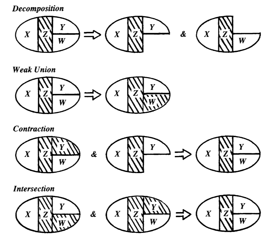
Theorem: (Pearl 2008) For disjoint subsets \(\mathbf{W},\mathbf{X},\mathbf{Y},\mathbf{Z}\subseteq\mathbf{V}.\)

Then the relation \(\cdot\perp\cdot|\cdot\) satisfies the following relations:

\[\begin{aligned} \mathbf{X} \perp \mathbf{Z} |\mathbf{Y} & \Leftrightarrow & \mathbf{Z}\perp \mathbf{X} | \mathbf{Y} && \text{ Symmetry }&\\ \mathbf{X} \perp \mathbf{Y}\cup \mathbf{W} |\mathbf{Z} & \Rightarrow & \mathbf{X} \perp \mathbf{Y} \text{ and } \mathbf{X} \perp \mathbf{W} && \text{ Decomposition }&\\ \mathbf{X} \perp \mathbf{Y}\cup \mathbf{W} |\mathbf{Z} & \Rightarrow & \mathbf{X} \perp \mathbf{Y}|\mathbf{Z}\cup\mathbf{W} && \text{ Weak Union }&\\ \mathbf{X} \perp \mathbf{Y} |\mathbf{Z} \text{ and } \mathbf{X} \perp \mathbf{W}|\mathbf{Z}\cup \mathbf{Y} |\mathbf{Z} & \Rightarrow & \mathbf{X} \perp \mathbf{Y}\cup \mathbf{W}|\mathbf{Z} && \text{ Contraction }&\\ \mathbf{X} \perp \mathbf{Y} |\mathbf{Z}\cup \mathbf{W} \text{ and } \mathbf{X} \perp \mathbf{W} |\mathbf{Z}\cup \mathbf{Y} & \Rightarrow & \mathbf{X}\perp \mathbf{W}\cup\mathbf{Y} | \mathbf{Z} && \text{ Intersection } & (*)\\ \end{aligned}\]

(*) The Intersection axiom only holds for strictly positive distributions.

visual intuition of graph axioms (Pearl 2008)

How can we relate this to the topology of the graph?

B in a fork path

B in a chain path

B in a collider path

Definition: A set \(\mathbf{S}\) blocks a path \(\pi\) from X to Y in a DAG \(\mathcal{G}\) if either

  1. There a node \(a\in\pi\) which is not a collider on \(\pi\) such that \(a\in\mathbf{S}\)

  2. There a node \(b\in\pi\) which is a collider on \(\pi\) and \(\operatorname{descendants}(b)\cap\mathbf{S}=\emptyset\)

If a path is not blocked, it is active.

Definition: A set \(\mathbf{S}\) d-separates two subsets of nodes \(\mathbf{X},\mathbf{X}\subseteq\mathcal{G}\) if it blocks every path between any every pair of nodes \((A,B)\) such that \(A\in\mathbf{X},\, B\in\mathbf{Y}.\)

This looks ghastly and unintuitive, but we have to live with it because it is the shortest path to making simple statements about conditional independence DAGs without horrible circumlocutions, or starting from undirected graphs, which is tedious.

Theorem: (Pearl 2008; Steffen L. Lauritzen 1996). If the joint distribution of \(\mathbf{V}\) factorises according to the DAG \(\mathbf{G}\) then for two subsets of variables \(\mathbf{X}\perp\mathbf{Y}|\mathbf{S}\) iff \(\mathbf{S}\) d-separates \(\mathbf{X}\) and \(\mathbf{Y}\).

This puts us in a position to make more intuitive statements about the conditional independence relationships that we may read off the DAG.

Corollary: The DAG Markov property.

\[ X \perp \operatorname{descendants}(X)^C|\operatorname{parents}(X) \]

Corollary: The DAG Markov blanket.

Define

\[ \operatorname{blanket}(X):= \operatorname{parents}(X)\cup \operatorname{children}(X)\cup \operatorname{coparents}(X) \]

Then

\[ X\perp \operatorname{blanket}(X)^C|\operatorname{blanket}(X) \]

Causal interpretation

We have a DAG \(\mathcal{G}\) and a set of variables \(\mathbf{V}\) to which we wish to give a causal interpretation.

Assume

  1. The \(\mathbf{V}\) factors according to \(\mathcal{G}\)
  2. \(X\rightarrow Y\) means “causes” (The Causal Markov property)
  3. We additionally assume faithfulness, that is, that \(X\leftrightsquigarrow Y\) iff there is a path connecting them.

So, are we done?

Correlation tastes as good as causation Messerli (2012)

We add the additional condition that

  1. all the relevant variables are included in the graph.

The BBC raised one possible confounding variable:

[…] Eric Cornell, who won the Nobel Prize in Physics in 2001, told Reuters “I attribute essentially all my success to the very large amount of chocolate that I consume. Personally I feel that milk chocolate makes you stupid… dark chocolate is the way to go. It’s one thing if you want a medicine or chemistry Nobel Prize but if you want a physics Nobel Prize it pretty much has got to be dark chocolate.”

do-calculus

Now we can discuss the relationship between conditional dependence and causal effect. This is the difference between, say,

\[ P(\text{Wet pavement}|\text{Sprinkler}=on) \]

and

\[ P(\text{Wet pavement}|\operatorname{do}(\text{Sprinkler}=on)). \]

This is called “truncated factorization” in the paper. \(\operatorname{do}\)-calculus and graph surgery give us rules that allow us to calculate dependencies under marginalisation for intervention distributions.

If we know \(P\), this is relatively easy. Marginalize out all influences to the causal variable of interest, which we show graphically as wiping out a link.

Now suppose we are not given complete knowledge of \(P\), but only some of the conditional distributions. (there are unobservable variables). This is the setup of observational studies and epidemiology and so on.

What variables must we know the conditional distributions of in order to know the conditional effect? That is, we call a set of covariates \(\mathbf{S}\) an admissible set (or sufficient set) with respect to identifying the effect of \(X\) on \(Y\) iff

\[ p(Y=y|\operatorname{do}(X=x))=\sum_{\mathbf{s}} P(Y=y|X=x,\mathbf{S}=\mathbf{s}) P(\mathbf{S}=\mathbf{s}). \]

Parent criterion
The parents of a cause are an admissible set (Pearl 2009a).
Back-door criterion

A set \(\mathbf{S}\) is sufficient if

  1. \(\mathbf{S}\cap\operatorname{descendants}(X)=\emptyset\)
  2. \(\mathbf{S}\) blocks all paths which start with an arrow into \(\mathbf{X}\)

There are other criteria.

Causal properties of sufficient sets:

\[ P(Y=y|\operatorname{do}(X=x),S=s)=P(Y=y|X=x,S=s) \]

Hence

\[ P(Y=y|\operatorname{do}(X=x),S=s)=\sum_sP(Y=y|X=x,S=s)P(S=s). \]

More graph transformation rules! But this time for interventions.

Rule 1 (Insertion/deletion of observations)
\(P(Y\mid \operatorname{do}(X),Z,W)=P(Y\mid \operatorname{do}(X),W)\) if \(Y\) and \(Z\) are d-separated by \(X\cup W\) in \(\mathcal{G}^*\), the graph obtained from \(\mathcal{G}\) by removing all arrows pointing into variables in \(X\).
Rule 2 (Action/observation exchange)
\(P(Y\mid \operatorname{do}(X),\operatorname{do}(Z),W)=P(Y\mid \operatorname{do}(X),Z,W)\) if \(Y\) and \(Z\) are d-separated by \(X\cup W\) in \(\mathcal{G}^{\dagger}\), the graph obtained from \(\mathcal{G}\) by removing all arrows pointing into variables in \(X\) and all arrows pointing out of variables in \(Z.\)
Rule 3 (Insertion/deletion of actions)
\(P(Y\mid \operatorname{do}(X),Z,W)=P(Y\mid \operatorname{do}(X),W)\) if \(Y\) and \(Z\) are d-separated by \(X\cup W\) in \(\mathcal{G}^{\ddagger}\), the graph obtained from \(\mathcal{G}\) by removing all arrows pointing into variables in \(X\) (thus creating \(\mathcal{G}^*\)) and then removing all of the arrows pointing into variables in \(Z\) that are not ancestors of any variable in \(W\) in \(\mathcal{G}^*.\)

If some causal effect of a DAG is identifiable, then there exists a sequence of application of the do-calculus rules that can identify causal effects using only observational quantities (Shpitser and Pearl 2008)

Case study: Causal GPs

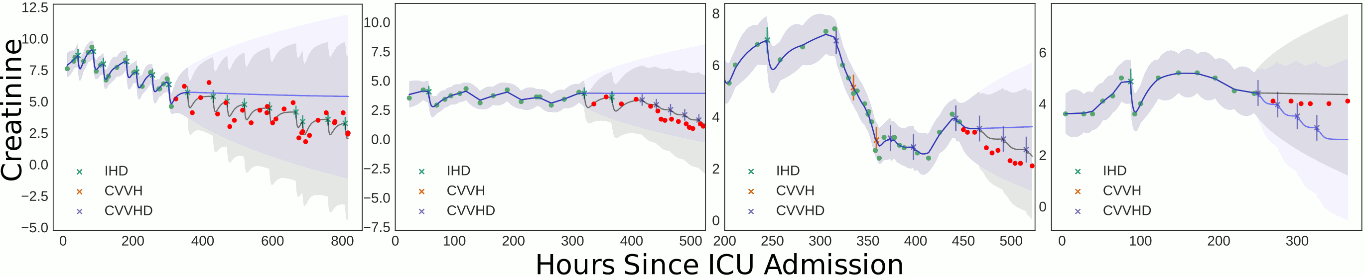
Here is a cute paper (Schulam and Saria 2017) on causal Gaussian process regression. You need the supplement to the paper for it to make sense.

It uses Gaussian process regression to infer a time series model without worrying about discretization which is tricky in alternative approaches (e.g. Brodersen et al. (2015)).

  1. (Consistency). Let \(Y\) be the observed outcome, \(A \in \mathcal{C}\) be the observed action, and \(Y[a]\) be the potential outcome for action \(a \in \mathcal{C},\) then: \((Y \triangleq Y[a]) \mid A=a\)
  2. (Continuous-Time NUC). For all times \(t\) and all histories \(\mathcal{H}_{t^{-}}\), the densities \(\lambda^{*}(t)\), \(p^{*}\left(z_{y}, z_{a} \mid t\right),\) and \(p^{*}\left(a \mid y, t, z_{a}\right)\) do not depend on \(Y_{s}[\) a \(]\) for all times \(s>t\) and all actions a.
  3. (Non-Informative Measurement Times). For all times t and any history \(\mathcal{H}_{t^{-}}\), the following holds: \(p^{*}\left(y \mid t, z_{y}=1\right) \mathrm{d} y=P\left(Y_{t} \in \mathrm{d} y \mid \mathcal{H}_{t^{-}}\right)\)

Schulam and Saria’s DAG

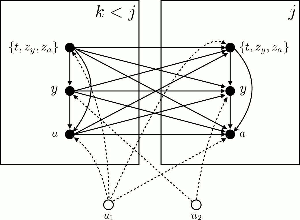
Notation decoder ring:

\[(Y[a]|X):= P(Y|X,\operatorname{do}(A=a)\]

What are unobserved \(u_1,u_2\)? Event and action models? Where are latent patience health states? \(u_2\) only effects outcome measurements. Why is there a point process at all? Does each patient possess a true latent class?

How does causality flow through GP?

Why is the latent mean 5-dimensional?

References

Aalen, Odd O, K Røysland, Jm Gran, R Kouyos, and T Lange. 2016. Can We Believe the DAGs? A Comment on the Relationship Between Causal DAGs and Mechanisms.” Statistical Methods in Medical Research 25 (5): 2294–314.
Aral, Sinan, Lev Muchnik, and Arun Sundararajan. 2009. Distinguishing Influence-Based Contagion from Homophily-Driven Diffusion in Dynamic Networks.” Proceedings of the National Academy of Sciences 106 (51): 21544–49.
Arnold, Barry C., Enrique Castillo, and Jose M. Sarabia. 1999. Conditional Specification of Statistical Models. Springer Science & Business Media.
Bareinboim, Elias, and Judea Pearl. 2016. Causal Inference and the Data-Fusion Problem.” Proceedings of the National Academy of Sciences 113 (27): 7345–52.
Bareinboim, Elias, Jin Tian, and Judea Pearl. 2014. Recovering from Selection Bias in Causal and Statistical Inference. In AAAI, 2410–16.
Bloniarz, Adam, Hanzhong Liu, Cun-Hui Zhang, Jasjeet Sekhon, and Bin Yu. 2015. Lasso Adjustments of Treatment Effect Estimates in Randomized Experiments.” arXiv:1507.03652 [Math, Stat], July.
Bongers, Stephan, Patrick Forré, Jonas Peters, Bernhard Schölkopf, and Joris M. Mooij. 2020. Foundations of Structural Causal Models with Cycles and Latent Variables.” arXiv:1611.06221 [Cs, Stat], October.
Bottou, Léon, Jonas Peters, Joaquin Quiñonero-Candela, Denis X. Charles, D. Max Chickering, Elon Portugaly, Dipankar Ray, Patrice Simard, and Ed Snelson. 2013. Counterfactual Reasoning and Learning Systems.” arXiv:1209.2355 [Cs, Math, Stat], July.
Brodersen, Kay H., Fabian Gallusser, Jim Koehler, Nicolas Remy, and Steven L. Scott. 2015. Inferring Causal Impact Using Bayesian Structural Time-Series Models.” The Annals of Applied Statistics 9 (1): 247–74.
Bühlmann, Peter. 2013. Causal Statistical Inference in High Dimensions.” Mathematical Methods of Operations Research 77 (3): 357–70.
Bühlmann, Peter, Markus Kalisch, and Lukas Meier. 2014. High-Dimensional Statistics with a View Toward Applications in Biology.” Annual Review of Statistics and Its Application 1 (1): 255–78.
Bühlmann, Peter, Jonas Peters, Jan Ernest, and Marloes Maathuis. 2014. Predicting Causal Effects in High-Dimensional Settings.”
Bühlmann, Peter, Philipp Rütimann, and Markus Kalisch. 2013. Controlling False Positive Selections in High-Dimensional Regression and Causal Inference.” Statistical Methods in Medical Research 22 (5): 466–92.
Chen, B, and J Pearl. 2012. “Regression and Causation: A Critical Examination of Econometric Textbooks.”
Claassen, Tom, Joris M. Mooij, and Tom Heskes. 2014. Proof Supplement - Learning Sparse Causal Models Is Not NP-Hard (UAI2013).” arXiv:1411.1557 [Stat], November.
Colombo, Diego, Marloes H. Maathuis, Markus Kalisch, and Thomas S. Richardson. 2012. Learning High-Dimensional Directed Acyclic Graphs with Latent and Selection Variables.” The Annals of Statistics 40 (1): 294–321.
De Luna, Xavier, Ingeborg Waernbaum, and Thomas S. Richardson. 2011. Covariate Selection for the Nonparametric Estimation of an Average Treatment Effect.” Biometrika, October, asr041.
Elwert, Felix. 2013. Graphical Causal Models.” In Handbook of Causal Analysis for Social Research, edited by Stephen L. Morgan, 245–73. Handbooks of Sociology and Social Research. Dordrecht: Springer Netherlands.
Ernest, Jan, and Peter Bühlmann. 2014. Marginal Integration for Fully Robust Causal Inference.” arXiv:1405.1868 [Stat], May.
Gelman, Andrew. 2010. Causality and Statistical Learning.” American Journal of Sociology 117 (3): 955–66.
Hinton, Geoffrey E., Simon Osindero, and Kejie Bao. 2005. Learning Causally Linked Markov Random Fields.” In Proceedings of the 10th International Workshop on Artificial Intelligence and Statistics, 128–35. Citeseer.
Hoyer, Patrik O., Dominik Janzing, Joris M Mooij, Jonas Peters, and Bernhard Schölkopf. 2009. Nonlinear Causal Discovery with Additive Noise Models.” In Advances in Neural Information Processing Systems 21, edited by D. Koller, D. Schuurmans, Y. Bengio, and L. Bottou, 689–96. Curran Associates, Inc.
Janzing, Dominik, Joris Mooij, Kun Zhang, Jan Lemeire, Jakob Zscheischler, Povilas Daniušis, Bastian Steudel, and Bernhard Schölkopf. 2012. Information-Geometric Approach to Inferring Causal Directions.” Artificial Intelligence 182-183 (May): 1–31.
Janzing, Dominik, and Bernhard Schölkopf. 2010. Causal Inference Using the Algorithmic Markov Condition.” IEEE Transactions on Information Theory 56 (10): 5168–94.
Jordan, Michael Irwin. 1999. Learning in Graphical Models. Cambridge, Mass.: MIT Press.
Jordan, Michael I., and Yair Weiss. 2002a. Graphical Models: Probabilistic Inference.” The Handbook of Brain Theory and Neural Networks, 490–96.
———. 2002b. Probabilistic Inference in Graphical Models.” Handbook of Neural Networks and Brain Theory.
Kalisch, Markus, and Peter Bühlmann. 2007. Estimating High-Dimensional Directed Acyclic Graphs with the PC-Algorithm.” Journal of Machine Learning Research 8 (May): 613–36.
Kennedy, Edward H. 2015. Semiparametric Theory and Empirical Processes in Causal Inference.” arXiv Preprint arXiv:1510.04740.
Kim, Jin H., and Judea Pearl. 1983. A Computational Model for Causal and Diagnostic Reasoning in Inference Systems. In IJCAI, 83:190–93. San Francisco, CA, USA: Citeseer.
Koller, Daphne, and Nir Friedman. 2009. Probabilistic Graphical Models : Principles and Techniques. Cambridge, MA: MIT Press.
Lauritzen, S. L., and D. J. Spiegelhalter. 1988. Local Computations with Probabilities on Graphical Structures and Their Application to Expert Systems.” Journal of the Royal Statistical Society. Series B (Methodological) 50 (2): 157–224.
Lauritzen, Steffen L. 1996. Graphical Models. Oxford Statistical Science Series. Clarendon Press.
———. 2000. Causal Inference from Graphical Models.” In Complex Stochastic Systems, 63–107. CRC Press.
Li, Yunzhu, Antonio Torralba, Animashree Anandkumar, Dieter Fox, and Animesh Garg. 2020. Causal Discovery in Physical Systems from Videos.” arXiv:2007.00631 [Cs, Stat], July.
Maathuis, Marloes H., and Diego Colombo. 2013. A Generalized Backdoor Criterion.” arXiv Preprint arXiv:1307.5636.
Maathuis, Marloes H., Diego Colombo, Markus Kalisch, and Peter Bühlmann. 2010. Predicting Causal Effects in Large-Scale Systems from Observational Data.” Nature Methods 7 (4): 247–48.
Maathuis, Marloes H., Markus Kalisch, and Peter Bühlmann. 2009. Estimating High-Dimensional Intervention Effects from Observational Data.” The Annals of Statistics 37 (6A): 3133–64.
Marbach, Daniel, Robert J. Prill, Thomas Schaffter, Claudio Mattiussi, Dario Floreano, and Gustavo Stolovitzky. 2010. Revealing Strengths and Weaknesses of Methods for Gene Network Inference.” Proceedings of the National Academy of Sciences 107 (14): 6286–91.
Meinshausen, Nicolai. 2018. Causality from a Distributional Robustness Point of View.” In 2018 IEEE Data Science Workshop (DSW), 6–10.
Messerli, Franz H. 2012. Chocolate Consumption, Cognitive Function, and Nobel Laureates.” New England Journal of Medicine 367 (16): 1562–64.
Mihalkova, Lilyana, and Raymond J. Mooney. 2007. Bottom-up Learning of Markov Logic Network Structure.” In Proceedings of the 24th International Conference on Machine Learning, 625–32. ACM.
Montanari, Andrea. 2011. Lecture Notes for Stat 375 Inference in Graphical Models.”
Mooij, Joris M., Jonas Peters, Dominik Janzing, Jakob Zscheischler, and Bernhard Schölkopf. 2016. Distinguishing Cause from Effect Using Observational Data: Methods and Benchmarks.” Journal of Machine Learning Research 17 (32): 1–102.
Morgan, Stephen L., and Christopher Winship. 2015. Counterfactuals and Causal Inference. Cambridge University Press.
Murphy, Kevin P. 2012. Machine learning: a probabilistic perspective. 1 edition. Adaptive computation and machine learning series. Cambridge, MA: MIT Press.
Nair, Suraj, Yuke Zhu, Silvio Savarese, and Li Fei-Fei. 2019. Causal Induction from Visual Observations for Goal Directed Tasks.” arXiv:1910.01751 [Cs, Stat], October.
Narendra, Tanmayee, Anush Sankaran, Deepak Vijaykeerthy, and Senthil Mani. 2018. Explaining Deep Learning Models Using Causal Inference.” arXiv:1811.04376 [Cs, Stat], November.
Nauta, Meike, Doina Bucur, and Christin Seifert. 2019. Causal Discovery with Attention-Based Convolutional Neural Networks.” Machine Learning and Knowledge Extraction 1 (1): 312–40.
Neapolitan, Richard E. 2003. Learning Bayesian Networks. Vol. 38. Prentice Hal, Paperback.
Ng, Ignavier, Shengyu Zhu, Zhitang Chen, and Zhuangyan Fang. 2019. A Graph Autoencoder Approach to Causal Structure Learning.” In Advances In Neural Information Processing Systems.
Noel, Hans, and Brendan Nyhan. 2011. The ‘Unfriending’ Problem: The Consequences of Homophily in Friendship Retention for Causal Estimates of Social Influence.” Social Networks 33 (3): 211–18.
Pearl, Judea. 1982. Reverend Bayes on Inference Engines: A Distributed Hierarchical Approach.” In Proceedings of the Second AAAI Conference on Artificial Intelligence, 133–36. AAAI’82. Pittsburgh, Pennsylvania: AAAI Press.
———. 1986. Fusion, Propagation, and Structuring in Belief Networks.” Artificial Intelligence 29 (3): 241–88.
———. 1998. Graphical Models for Probabilistic and Causal Reasoning.” In Quantified Representation of Uncertainty and Imprecision, edited by Philippe Smets, 367–89. Handbook of Defeasible Reasoning and Uncertainty Management Systems. Dordrecht: Springer Netherlands.
———. 2008. Probabilistic reasoning in intelligent systems: networks of plausible inference. Rev. 2. print., 12. [Dr.]. The Morgan Kaufmann series in representation and reasoning. San Francisco, Calif: Kaufmann.
———. 2009a. Causal Inference in Statistics: An Overview.” Statistics Surveys 3: 96–146.
———. 2009b. Causality: Models, Reasoning and Inference. Cambridge University Press.
Peters, Jonas, Peter Bühlmann, and Nicolai Meinshausen. 2015. Causal Inference Using Invariant Prediction: Identification and Confidence Intervals.” arXiv:1501.01332 [Stat], January.
Raginsky, M. 2011. Directed Information and Pearl’s Causal Calculus.” In 2011 49th Annual Allerton Conference on Communication, Control, and Computing (Allerton), 958–65.
Richardson, Thomas, and Peter Spirtes. 2002. Ancestral Graph Markov Models.” Annals of Statistics 30 (4): 962–1030.
Robins, James M. 1997. Causal Inference from Complex Longitudinal Data.” In Latent Variable Modeling and Applications to Causality, edited by Maia Berkane, 69–117. Lecture Notes in Statistics. New York, NY: Springer.
Rubenstein, Paul K., Sebastian Weichwald, Stephan Bongers, Joris M. Mooij, Dominik Janzing, Moritz Grosse-Wentrup, and Bernhard Schölkopf. 2017. Causal Consistency of Structural Equation Models.” arXiv:1707.00819 [Cs, Stat], July.
Rubin, Donald B, and Richard P Waterman. 2006. Estimating the Causal Effects of Marketing Interventions Using Propensity Score Methodology.” Statistical Science 21 (2): 206–22.
Sauer, Brian, and Tyler J. VanderWeele. 2013. Use of Directed Acyclic Graphs. Agency for Healthcare Research and Quality (US).
Schulam, Peter, and Suchi Saria. 2017. Reliable Decision Support Using Counterfactual Models.” In Proceedings of the 31st International Conference on Neural Information Processing Systems, 1696–706. NIPS’17. Red Hook, NY, USA: Curran Associates Inc.
Shalizi, Cosma Rohilla, and Edward McFowland III. 2016. Controlling for Latent Homophily in Social Networks Through Inferring Latent Locations.” arXiv:1607.06565 [Physics, Stat], July.
Shalizi, Cosma Rohilla, and Andrew C. Thomas. 2011. Homophily and Contagion Are Generically Confounded in Observational Social Network Studies.” Sociological Methods & Research 40 (2): 211–39.
Shpitser, Ilya, and Judea Pearl. 2008. “Complete Identification Methods for the Causal Hierarchy.” The Journal of Machine Learning Research 9: 1941–79.
Shpitser, Ilya, and Eric Tchetgen Tchetgen. 2014. Causal Inference with a Graphical Hierarchy of Interventions.” arXiv:1411.2127 [Stat], November.
Shrier, Ian, and Robert W. Platt. 2008. Reducing Bias Through Directed Acyclic Graphs.” BMC Medical Research Methodology 8 (1): 70.
Smith, David A., and Jason Eisner. 2008. Dependency Parsing by Belief Propagation.” In Proceedings of the Conference on Empirical Methods in Natural Language Processing, 145–56. Association for Computational Linguistics.
Smith, Gordon C. S., and Jill P. Pell. 2003. Parachute Use to Prevent Death and Major Trauma Related to Gravitational Challenge: Systematic Review of Randomised Controlled Trials.” BMJ 327 (7429): 1459–61.
Spirtes, Peter, Clark Glymour, and Richard Scheines. 2001. Causation, Prediction, and Search. Second Edition. Adaptive Computation and Machine Learning. The MIT Press.
Subbaswamy, Adarsh, Peter Schulam, and Suchi Saria. 2019. Preventing Failures Due to Dataset Shift: Learning Predictive Models That Transport.” In The 22nd International Conference on Artificial Intelligence and Statistics, 3118–27. PMLR.
Textor, Johannes, and Maciej Liśkiewicz. 2011. Adjustment Criteria in Causal Diagrams: An Algorithmic Perspective.” In Proceedings of the Twenty-Seventh Conference on Uncertainty in Artificial Intelligence, 681–88. UAI’11. Arlington, Virginia, USA: AUAI Press.
Vansteelandt, Stijn, Maarten Bekaert, and Gerda Claeskens. 2012. On Model Selection and Model Misspecification in Causal Inference.” Statistical Methods in Medical Research 21 (1): 7–30.
Weichwald, Sebastian, and Jonas Peters. 2020. Causality in Cognitive Neuroscience: Concepts, Challenges, and Distributional Robustness.” arXiv:2002.06060 [q-Bio, Stat], July.
Wright, Sewall. 1934. The Method of Path Coefficients.” The Annals of Mathematical Statistics 5 (3): 161–215.
Yedidia, J.S., W.T. Freeman, and Y. Weiss. 2003. Understanding Belief Propagation and Its Generalizations.” In Exploring Artificial Intelligence in the New Millennium, edited by G. Lakemeyer and B. Nebel, 239–36. Morgan Kaufmann Publishers.
Zander, Benito van der, and Maciej Liśkiewicz. 2016. Separators and Adjustment Sets in Markov Equivalent DAGs.” In Proceedings of the Thirtieth AAAI Conference on Artificial Intelligence, 3315–21. AAAI’16. Phoenix, Arizona: AAAI Press.
Zander, Benito van der, Maciej Liśkiewicz, and Johannes Textor. 2014. Constructing Separators and Adjustment Sets in Ancestral Graphs.” In Proceedings of the UAI 2014 Conference on Causal Inference: Learning and Prediction - Volume 1274, 11–24. CI’14. Aachen, DEU: CEUR-WS.org.
Zander, Benito van der, Johannes Textor, and Maciej Liskiewicz. 2015. Efficiently Finding Conditional Instruments for Causal Inference.” In Proceedings of the 24th International Conference on Artificial Intelligence, 3243–49. IJCAI’15. Buenos Aires, Argentina: AAAI Press.
Zhang, Kun, Jonas Peters, Dominik Janzing, and Bernhard Schölkopf. 2012. Kernel-Based Conditional Independence Test and Application in Causal Discovery.” arXiv:1202.3775 [Cs, Stat], February.

  1. Terminology confusion: This is orthogonal to subjective probability.↩︎


No comments yet. Why not leave one?

GitHub-flavored Markdown & a sane subset of HTML is supported.